Phase Response in Active Filters: The Band-Pass Response

While filters are designed primarily for their amplitude response, the phase response can be important in some applications.

Introduction

In the first article of this series, I examined the relationship of the filter phase to the topology of the implementation of the filter. In the second article, I examined the phase shift of the filter transfer function for the low-pass and high-pass responses. This article will concentrate on the band-pass response. While filters are designed primarily for their amplitude response, the phase response can be important in some applications.

For purposes of review, the transfer function of an active filter is actually the cascade of the filter transfer function and the amplifier transfer function (see Figure 1).

 

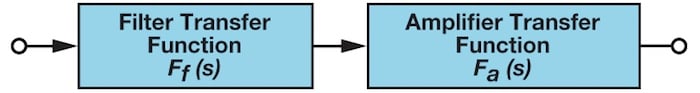
Figure 1. Filter as cascade of two transfer functions.

The Band-Pass Transfer Function

Changing the numerator of the low-pass prototype to

 

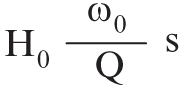
will convert the filter to a band-pass function. This will put a zero in the transfer function. An s term in the numerator gives us a zero and an s term in the numerator gives us a pole. A zero will give a rising response with frequency while a pole will give a falling response with frequency.

The transfer function of a second-order band-pass filter is then:

 

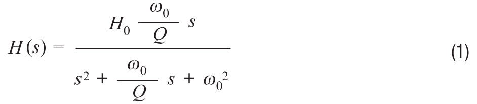
ω0 here is the frequency (F0 = 2 π ω0) at which the gain of the filter peaks.

H0 is the circuit gain (Q peaking) and is defined as:

 

where H is the gain of the filter implementation.

Q has a particular meaning for the band-pass response. It is the selectivity of the filter. It is defined as:

 

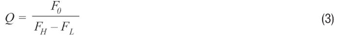
where FL and FH are the frequencies where the response is –3 dB from the maximum.

The bandwidth (BW) of the filter is described as:

 

It can be shown that the resonant frequency (F0) is the geometric mean of FL and FH, which means that F0 will appear half way between FL and FH on a logarithmic scale.

 

Also, note that the skirts of the band-pass response will always be symmetrical around F0 on a logarithmic scale.

The amplitude response of a band-pass filter to various values of Q is shown in Figure 2. In this figure, the gain at the center frequency is normalized to 1 (0 dB).

 

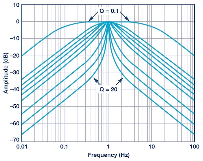
Figure 2. Normalized band-pass filter amplitude response.

Again, this article is primarily concerned with the phase response, but it is useful to have an idea of the amplitude response of the filter.

A word of caution is appropriate here. Band-pass filters can be defined two different ways. The narrow-band case is the classic definition that we have shown above. In some cases, however, if the high and low cutoff frequencies are widely separated, the band-pass filter is constructed out of separate high-pass and low-pass sections. Widely separated, in this context, means separated by at least two octaves (×4 in frequency). This is the wideband case. We are primarily concerned with the narrow-band case for this article. For the wideband case, evaluate the filter as separate high-pass and low-pass sections.

While a band-pass filter can be defined in terms of standard responses, such as Butterworth, Bessel, or Chebyshev, they are also commonly defined by their Q and F0.

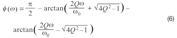
The phase response of a band-pass filter is:

 

Note that there is no such thing as a single-pole band-pass filter.

 

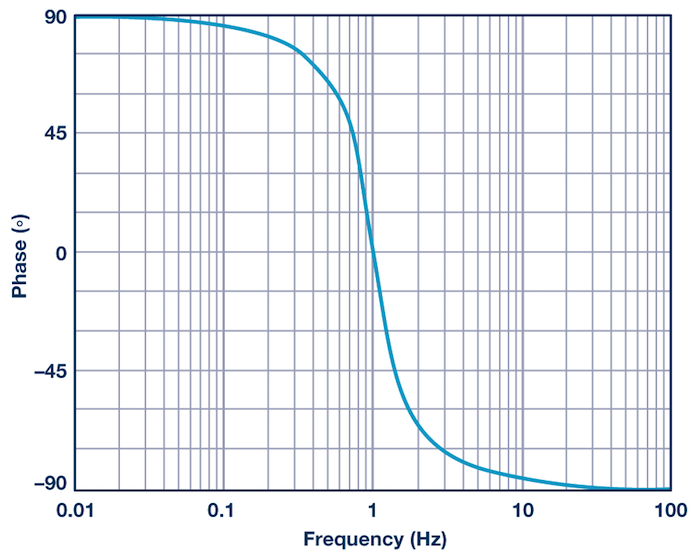
Figure 3. Normalized band-pass filter phase response.

Figure 3 evaluates Equation 6 from two decades below the center frequency to two decades above the center frequency. The center frequency has a phase shift of 0°. The center frequency is 1 and the Q is 0.707. This is the same Q used in the previous article, although in that article we used α. Remember α = 1/Q.

Inspection shows the shape of this curve is basically the same as that of the low-pass (and the high-pass for that matter). In this case, however, the phase shift is from 90°, below the center frequency going to 0° at the center frequency to –90° above the center frequency.

In Figure 4 we examine the phase response of the band-pass filter with varying Q. If we take a look at the transfer function, we can see that the phase change can take place over a relatively large frequency range, and that the range of the change is inversely proportional to the Q of the circuit. Again, inspection shows that the curves have the same shape as those for the low-pass (and high-pass) responses, just with a different range.

 

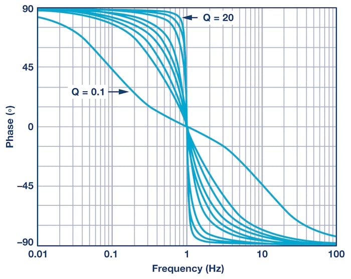
Figure 4. Normalized band-pass filter phase response with varying Q.

The Amplifier Transfer Function

It has been shown in previous installments that the transfer function is basically that of a single-pole filter. While the phase shift of the amplifier is generally ignored, it can affect the overall transfer of the composite filter. The AD822 was arbitrarily chosen to use in the simulations of the filters in this article. It was chosen partially to minimize the effect on the filter transfer function. This is because the phase shift of the amplifier is considerably higher in frequency than the corner frequency of the filter itself. The transfer function of the AD822 is shown in Figure 5, which is information taken directly from the data sheet.

 

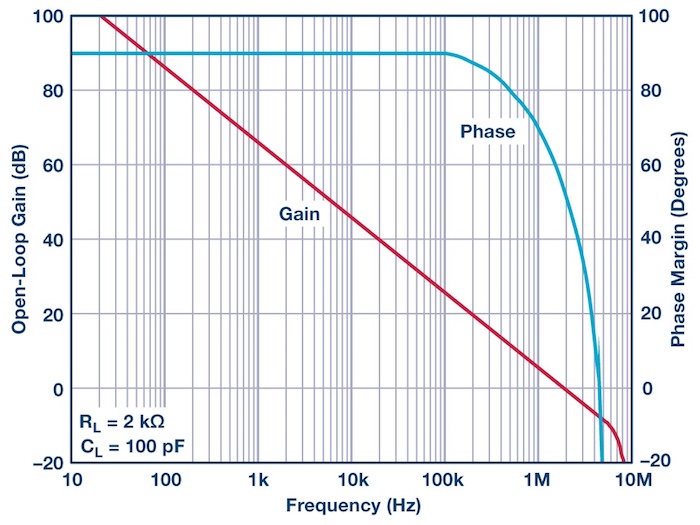
Figure 5. AD822 bode plot gain and phase.

Example 1: A 1 kHz, 2-Pole Band-Pass Filter with a Q = 20

The first example will be a filter designed as a band-pass from the start. We arbitrarily choose a center frequency of 1 kHz and a Q of 20. Since the Q is on the higher side, we will use the dual amplifier band-pass (DABP) configuration. Again, this is an arbitrary choice.

We use the design equations from Reference 1. The resultant circuit is shown in Figure 6:

 

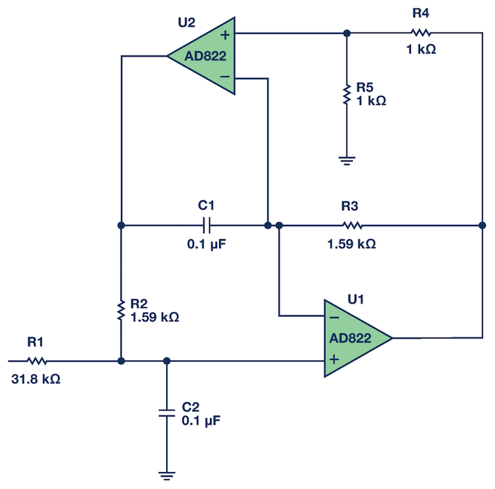
Figure 6. 1 kHz, Q = 20 DABP band-pass filter.

We are primarily concerned with phase in this article, but I think it useful to examine the amplitude response.

 

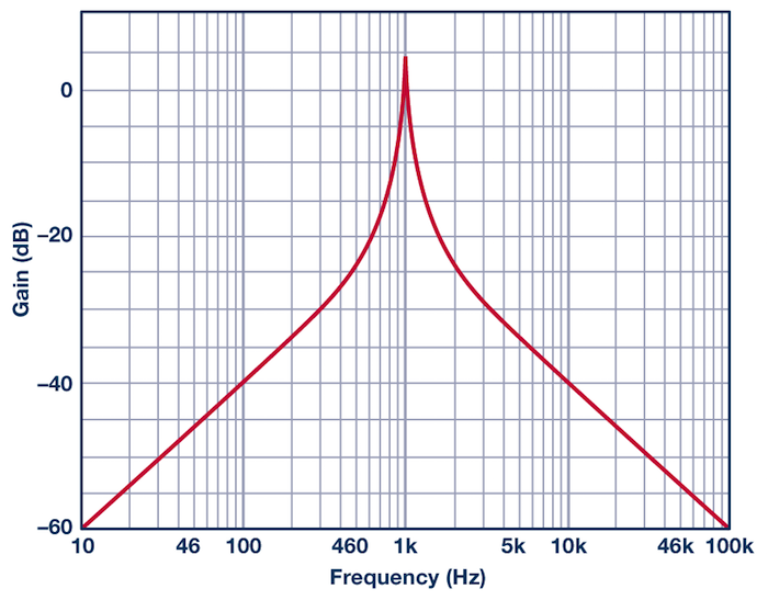
Figure 7. 1 kHz, Q = 20 DABP band-pass filter amplitude response.

We see the phase response in Figure 8:

 

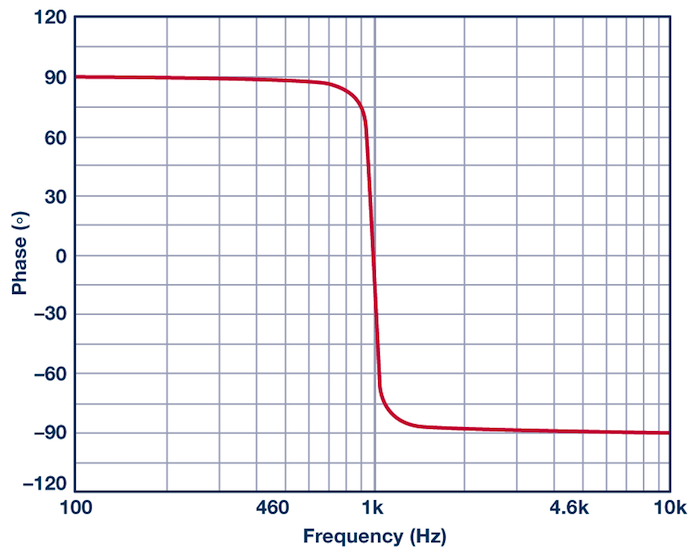
Figure 8. 1 kHz, Q = 20 DABP band-pass filter phase response.

Note that the DABP configuration is noninverting. Figure 8 matches Figure 3.

Example 2: A 1 kHz, 3-Pole 0.5 dB Chebyshev Low-Pass to Band-Pass Filter Transformation

Filter theory is based on a low-pass prototype that can then be manipulated into the other forms. In this example, the prototype that will be used is a 1 kHz, 3-pole, 0.5 dB Chebyshev filter. A Chebyshev filter was chosen because it would show more clearly if the responses were not correct. The ripples in the pass band, for instance, would not line up. A Butterworth filter would probably be too forgiving in this instance. A 3-pole filter was chosen so that a pole pair and a single pole would be transformed.

The pole locations for the LP prototype (from Reference 1) are:

 

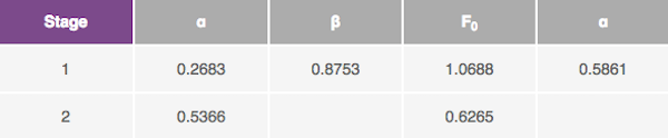
The first stage is the pole pair and the second stage is the single pole. Note the unfortunate convention of using α for two entirely separate parameters. The α and β on the left are the pole locations in the s plane. These are the values that are used in the transformation algorithms. The α on the right is 1/Q, which is what the design equations for the physical filters want to see.

The low-pass prototype is now converted to a band-pass filter. The equation string outlined in Reference 1 is used for the transformation. Each pole of the prototype filter will transform into a pole pair. Therefore, the 3-pole prototype, when transformed, will have six poles (3-pole pairs). In addition, there will be six zeros at the origin. There is no such thing as a single-pole band-pass.

Part of the transformation process is to specify the 3 dB bandwidth of the resultant filter. In this case, this bandwidth will be set to 500 Hz. The results of the transformation yield:

 

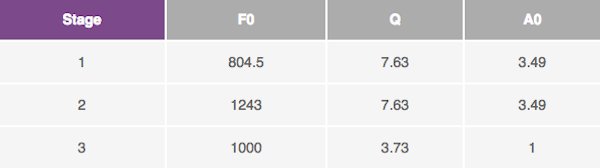
In practice, it might be useful to put the lower gain, lower Q section first in the string, to maximize signal level handling. The reason for the gain requirement for the first two stages is that their center frequencies will be attenuated relative to the center frequency of the total filter (that is, they will be on the skirt of other sections).

Since the resultant Qs are moderate (less than 20), the multiple feedback topology will be chosen. The design equations for the multiple feedback band-pass filter from Reference 1 are used to design the filter. Figure 9 shows the schematic of the filter itself.

 

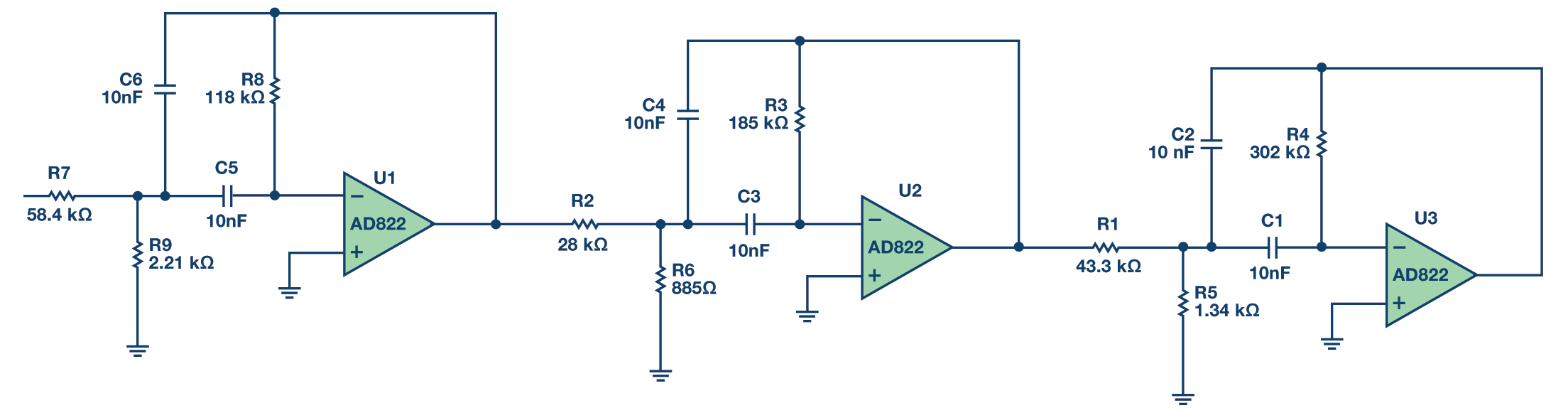
Figure 9. 1 kHz, 6-pole, 0.5 dB Chebyshev band-pass filter. Full-size image here.

In Figure 10 we look at the phase shift of the complete filter. The graph shows the phase shift of the first section alone (Section 1), of the first two sections together (Section 2), and of the complete filter (Section 3). These show the phase shift of the "real" filter sections, including the phase shift of the amplifier and the inversion of the filter topology.

There are a couple of details to note on Figure 10. First, the phase response is cumulative. The first section shows a change in phase of 180° (the phase shift of the filter function, disregarding the phase shift of the filter topology). The second section shows a phase change of 360° due to having two sections, 180° from each of the two sections. Remember that 360° = 0°. And the third section shows 540° of phase shift, 180° from each of the sections. Also note that at the frequencies above 10 kHz we are starting to see the phase roll-off slightly due to the amplifier response. We can see that the roll-off is again cumulative, increasing for each section.

 

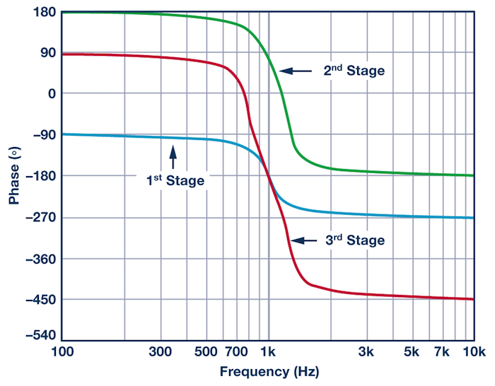
Figure 10. Phase response of a 1 kHz, 6-pole, 0.5 dB Chebyshev band-pass filter.

In Figure 11 we see the amplitude response of the complete filter.

 

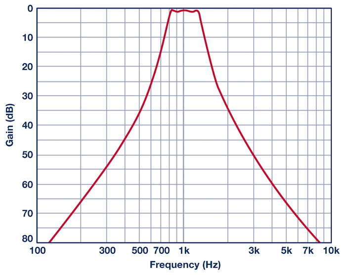
Figure 11. Amplitude response of a 1 kHz, 6-pole, 0.5 dB Chebyshev band-pass filter.

Conclusion

This article considers the phase shift of band-pass filters. In previous articles in this series, we examined the phase shift in relation to filter topology and for high-pass and low-pass topologies. In future articles, we will look at notch and all-pass filters. In the final installment, we will tie it all together and examine how the phase shift affects the transient response of the filter, looking at the group delay, impulse response, and step response, and what that means to the signal.

Further Reading

This article was originally published by Analog Dialogue. Visit their website to view more technical articles.

References

Daryanani, G. Principles of Active Network Synthesis and Design. John Wiley & Sons, 1976.

Graeme, J., G. Tobey, and L. Huelsman. Operational Amplifiers Design and Applications. McGraw-Hill, 1971.

Van Valkenburg, Mac. Analog Filter Design. Holt, Rinehart and Winston, 1982.

Williams, Arthur B. Electronic Filter Design Handbook. McGraw-Hill, 1981.

Zumbahlen, Hank. Basic Linear Design. Ch. 8. Analog Devices, Inc, 2006.

Zumbahlen, Hank. "Chapter 5: Analog Filters." Op Amp Applications Handbook. Newnes-Elsevier, 2006.

Zumbahlen, Hank. Linear Circuit Design Handbook. Newnes-Elsevier, 2008.

Zumbahlen, Hank. "Phase Relations in Active Filters." Analog Dialogue, Volume 41, 2007

Zverev, Anatol I. Handbook of Filter Synthesis. John Wiley & Sons, 1967.

Industry Articles are a form of content that allows industry partners to share useful news, messages, and technology with All About Circuits readers in a way editorial content is not well suited to. All Industry Articles are subject to strict editorial guidelines with the intention of offering readers useful news, technical expertise, or stories. The viewpoints and opinions expressed in Industry Articles are those of the partner and not necessarily those of All About Circuits or its writers.