Ambient Light Monitor: Measuring and Interpreting Ambient Light Levels
Part 3 in the “How to Make an Ambient Light Monitor” series. The project continues by building an ambient light sensor circuit on a breadboard, digitizing the circuit’s output signals, and interpreting the digitized measurements.
Part 3 in the “How to Make an Ambient Light Monitor” series.
Recommended Level
Beginner/Intermediate
Previous Articles in This Series
- Ambient Light Monitor: Display Measurements on an LCD
- Ambient Light Monitor: Understanding and Implementing the ADC
Required Hardware/Software
- SLSTK2000A EFM8 evaluation board
- Simplicity Studio integrated development environment
- Components listed in BOM
| Description | Quantity | Digi-Key p/n |
| Breadboard | 1 | 377-2094-ND |
| Receptacle-to-plug jumper wires | 3 | 1471-1231-ND |
| Ambient light detector | 1 | 425-2778-ND |
| 4.7 kΩ resistor | 1 | 4.7KQBK-ND |
| General purpose op-amp | 1 | LT1638CN8#PBF-ND |
| 0.1 µF capacitors | 2 | 399-4266-ND |
Project Overview
Previous articles discussed how to display current and voltage measurements on the LCD and how to perform reliable analog-to-digital conversions. We will now continue this project by building an ambient light sensor circuit on a breadboard, digitizing the circuit’s output signals, and interpreting the digitized measurements.
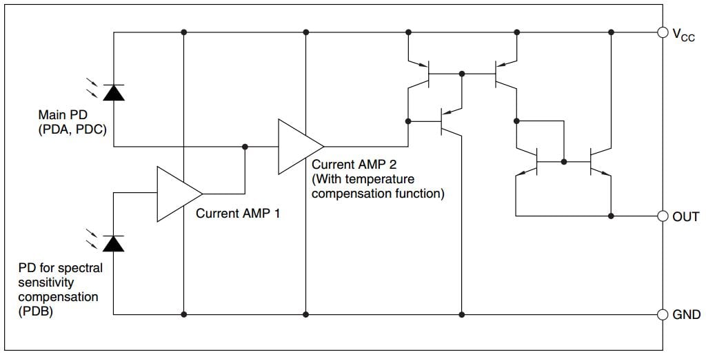
The light-sensitive component we will use is the GA1A2S100 Linear Output Ambient Light Sensor manufactured by SHARP. This three-terminal device is not a simple photodiode or phototransistor. Rather, it incorporates three photodiodes and conditioning circuitry, as follows:
The end result is a device whose sensitivity to light levels and spectral components is similar to that of the human eye. In other words, the output from this sensor gives a reasonably accurate indication of how light or dark an environment would appear to a human being.
The sensor generates an output current that is proportional to the ambient light level:

We need to pass this current through a load resistor to generate a voltage that can be measured by the EFM8’s ADC, so the first design task is sizing the load resistor. The sensor’s datasheet states that the voltage at the output pin should not exceed VCC - 1 V; we are using VCC = 3.3 V, so we need to choose a resistor that will produce about 2.3 V when the sensor is exposed to the highest expected light level. As indicated in the plot of output current vs. illuminance, the sensor is usable up to 10,000 lux. However, 10,000 lux is equivalent to being outside on a very cloudy day, which (interestingly) is far brighter than any normal indoor illuminance. Since this project is intended for monitoring indoor light levels, we will assume a maximum illuminance of 1000 lux (a well-lit office might be 500 lux). Looking at the above plot, we see that 1000 lux corresponds to 500 μA, and 2.3 V divided by 500 μA equals 4600 Ω. So we will choose a standard 4.7 kΩ resistor to convert the sensor’s output current into a voltage.
As we observed in the previous article, the input impedance of the ADC can interact with a circuit in a way that leads to erroneous measurements. This project does not suffer from two problematic factors that were present in the previous project: the external circuit does not include large amounts of series resistance, and there is no need to change the multiplexer setting because we are using only one analog input. Thus, settling time is not a major concern in this project. Nonetheless, we will still include an op-amp to buffer the sensor’s output, because this is a simple way to ensure that we have a low-impedance driver that can quickly charge the ADC’s sampling capacitor. As another benefit, with an op-amp in the circuit we could easily incorporate additional gain or a low-pass filter for suppressing unwanted high-frequency variations. In this project, though, we don’t need more gain and we will filter the measurements via firmware, so the op-amp is configured as a unity-gain buffer. Also, we don’t need to worry much about the op-amp doing more harm than good because its offset voltage and noise will not have a significant effect. The overall circuit is as follows:


Firmware
All the port I/O, peripheral, and interrupt configuration is the same as what we used in the previous article. The only changes are to the code in “AmbientLightMonitor_main.c”:
ADCFactor = (float)ADC_VREF_MILLIVOLTS/ADC_2POWER10;

SFRPAGE = ADC0_PAGE;
ADC0MX = ADCMUXIN_P1_1;

NumberofMeasurements = 0;
RawADCResult = 0;

while(1)
{
	ADC0CN0_ADBUSY = START_CONV;

	//wait until the conversion is complete
	while(ADC_CONV_COMPLETE == FALSE);
	ADC_CONV_COMPLETE = FALSE;

	//retrieve the 10-bit ADC value and add it to the accumulating sum in RawADCResult
	SFRPAGE = ADC0_PAGE;
	RawADCResult = RawADCResult + ADC0;
	NumberofMeasurements++;

	/*if we have enough measurements to compute an average,
	shift right to divide the sum by the number of measurements*/
	if(NumberofMeasurements == TWO_POWER_5)
	{
		RawADCResult = RawADCResult >> 5;
		NumberofMeasurements = 0;

		//convert the averaged conversion result to a current measurement and display
		//the actual value of the resistor in the test circuit is 4.6 kOhms
		ADCMeasurement = (RawADCResult*ADCFactor)/4.6;
		ConvertMeasurementandDisplay(CURRENT, ADCMeasurement);
	}

	//delay for 1/32 second so that we get one averaged measurement per second
	SFRPAGE = TIMER3_PAGE; TMR3 = 0; while(TMR3 < (10000/TWO_POWER_5));
}
The ADC multiplexer is set to P1.1 outside the while loop, because we have only one ADC input signal. Conversions are initiated by writing logic 1 (here represented by the preprocessor definition START_CONV) to the ADBUSY bit. Then we wait for the ADC_CONV_COMPLETE flag, which is set in the ADC interrupt service routine.
In this project, the ADC value is not immediately interpreted as a measurement and displayed. Instead, we implement a simple averaging filter. If you modify this code to display every conversion result, you may notice quite a bit of low-amplitude variation. This is caused by circuit noise and the relatively low resolution of the 10-bit ADC, though it also seems that the GA1A2S100 is susceptible to less-than-steady measurements, perhaps caused by subtle variations in sunlight reflecting in through windows. In any event, our ambient light monitor is intended to assess long-term trends in the illuminance of an indoor environment, so we will refine our measurements by displaying the average value of 32 consecutive samples. This is why we use the statement “RawADCResult = RawADCResult + ADC0”; the RawADCResult variable starts at zero and accumulates conversion results until the number of accumulated measurements equals 32, represented by the preprocessor definition TWO_POWER_5. The number of measurements used for the averaging filter should be an integer power of two, because this allows us to perform the division using an efficient bitwise shift-right operation. Also, we need to ensure that the accumulated ADC results will not exceed the maximum value of RawADCResult, which as an unsigned 16-bit variable will overflow beyond 65,535. The 10-bit ADC result can theoretically be as high as 1023, so 64 measurements would be close but acceptable (64 × 1023 = 65,472) and 128 would be way too many (128 × 1023 = 130,944).
The delay between displayed (i.e., averaged) measurements is always one second, regardless of how many samples we choose to average. This is accomplished with the “while(TMR3 < (10000/TWO_POWER_5))” statement: 10,000 Timer3 clocks correspond to one second, so dividing 10,000 by the number of averaged samples means that the delay between individual ADC conversions will produce samples at a rate that ensures one averaged measurement per second. Keep in mind that this update rate is still rather fast from a practical standpoint—if we were using these measurements to control a lamp dimmer, we would not want to dim the lights every time someone casts a temporary shadow on the optical sensor. But for now we simply want to observe the measurements, and with once-per-second updates we can better assess and ponder the sensor’s responsivity.
By the way, you may be wondering why we were determined to use an efficient bitwise shift operation (instead of division) when calculating the average, if we so casually use (10000/TWO_POWER_5) to calculate every single delay. The answer is that the compiler’s optimizer will recognize (10000/TWO_POWER_5) as a constant expression and produce assembly code that uses the corresponding constant quotient. The program loaded into the EFM8 will not actually perform a division here.
The ADC result represents a voltage, but we want to know the current generated by the GA1A2S100. To do this we must divide the voltage by the load resistor discussed above. One easy way to make our measurement a little more accurate is to use the actual value of the resistor rather than the nominal value. In the test circuit, the 4.7 kΩ resistor was actually 4.6 kΩ, so this is the value used in the code—i.e., “ADCMeasurement = (RawADCResult*ADCFactor)/4.6”; we use 4.6 instead of 4600 because the ConvertMeasurementandDisplay() function effectively incorporates division by 1000 when it interprets voltages as millivolts but currents as microamps.
Analysis
The basic functionality of the circuit can be readily confirmed by watching the measurements decrease as you cover the sensor with your thumb and then increase as you illuminate it with a lamp at close range. A more in-depth assessment requires equating measured output current to illuminance using the output current vs. illuminance plot above. It was fortunate that this circuit was tested on a pleasantly thuderstormy day in a room with six windows that admit a substantial amount of indirect sunlight. Artificial lighting was not used, and thus the slow, irregular procession of dark clouds mingled with early-August sunshine produced excellent variations in the indoor light level.
Occasionally the measurements moderately increased when the light level seemed to moderately decrease (or vice versa), perhaps owing to changes in spectral composition interacting unfavorably with the device’s “spectral sensitivity compensation” circuitry. And there is no doubt that successful implementation would require careful installation, because changes in the location or orientation of the sensor—e.g., closer to the floor, farther from the floor, directed toward a window, directed toward the ceiling—greatly affect the output. The performance would probably be more predictable in a windowless, uniformly lit office. Nevertheless, the GA1A2S100 responded well, its output current varying in a way that seemed consistent with the room’s general feeling of “lightness” or “darkness” or, at other times, with the level of illuminance one would expect based on the time of day. The latter relationship is more important if the primary goal is to conserve energy by adjusting indoor lighting in accordance with the amount of illumination provided by the sun. The current levels were typically in the range of 50 to 160 µA, corresponding to 100 to 300 lux. This range is consistent with expectations, considering that a well-lit residential room might be somewhere from 200 to 700 lux.
Video
Next Article in Series: Ambient Light Monitor: Zero-Cross Detection
Give this project a try for yourself! Get the BOM.