Derive and Plot a Low Pass Transfer Function on MATLAB

Become an Akerberg-Mossberg Filters champion.

Introduction to Filters

A filter is a circuit that removes unwanted frequencies from a waveform. Filters can be used to remove noise from a system to make it cleaner. It consists of two main bands: the pass band and the stop band.

To understand the pass band and stop band in a filter, we need to understand Bode plots. A Bode plot is a graph that tracks the response of frequencies. It shows the magnitude of a signal with respect to the frequency. The magnitude or the amplitude is measured in decibels and plotted on the Y-axis of the Bode plot. The X-axis of the bode plot is the frequency of the filter. 

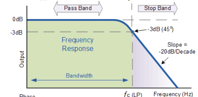
Figure 1. Example of a Low Pass Bode Plot

The above image is a bode plot for a low pass filter. The frequencies in the pass band are the frequencies with an amplitude of 0 decibels or above. The frequencies after the cutoff frequencies f_c are in the stop band. The frequencies that we want to remove would be in the stop band when the magnitude is less than zero.  

Depending on which frequencies we want to remove, the location of the pass band will vary to create the main 4 filters types. The main four filter response types are:

• High pass filters
• Low pass filters
• Band pass filters
• Band stop filters

The order of a filter indicates how steep the slope is. For every raise in order of a filter, there is a 6db/octave increase in the filter’s slope. An ideal perfect filter would have a slope of infinity. It would look like a square wave. Unfortunately, these ideal filters cannot be made in real life, and we can only make filters that have a roll-off or slope as close to this as we can. 

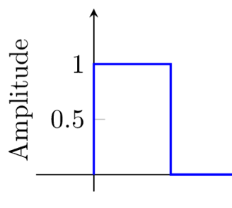
Figure 2. Frequency response of an Ideal Filter

Akerberg-Mossberg Biquad Filter

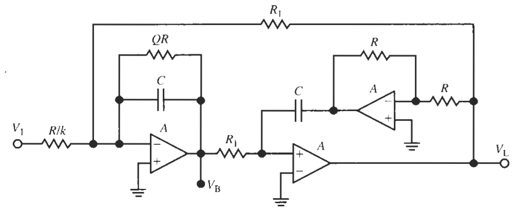
Figure 3. Akerberg Mossberg Filter

The Akerberg-Mossberg Filter as seen in Figure 3 is a Miller Integrator with a non-inverting integrator in the output. The advantages of using an Akerberg-Mossberg Filter is that the designing of it is easier and the Q (Quality Factor of the Frequency Response) is more predictable and the error in the gain is minimized. The normalized version of the Akerberg-Mossberg Circuit above will need a summing configuration to be able to design a circuit and plot it on MATLAB.

The summing circuit at the end of the Akerberg-Mossberg will look like this:

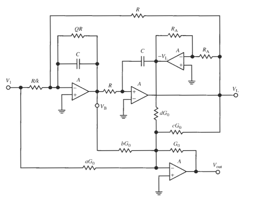
Figure 4. The Akerberg-Mossberg Filter with a summing circuit added

The summer adds the input signals and the signal from the band pass and low pass outputs. For the Ackerberg-Mossberg with a summing circuit the Transfer Function is the following equation below. 

Equation 1. General transfer function of the Akerberg-Mossberg with a summing circuit

Now with this transfer function, we have 5 variables that we can play with to obtain our desired frequency response. Our 5 Variables are a, b, c, d and k. We will only be manipulating these variables to change the numerator; our denominator will stay the same. With this transfer function, we can derive the transfer function for all types of filters like low pass, high pass, band pass, band stop, all pass, low pass notch and a high pass notch. 

Deriving a Low Pass Transfer Function

The transfer function for a low pass Akerberg-Mossberg filter is seen below in equation 2. 

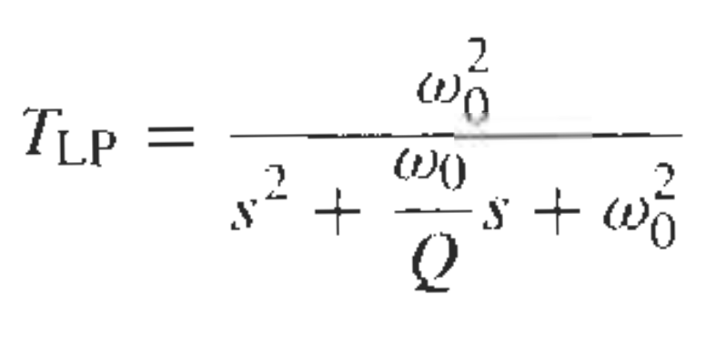
Equation 2. Low Pass Ackerberg Mossberg

Now we have to find the correct values for a,b,c, and d in equation 1 to end up with the transfer function of the low pass filter. We see that the numerator that we want only has w₀² so we have to get rid of the other monomials to only leave w₀² by itself. The first variable we want to get rid of is the first term, as². So we set a=0 in this case. The second terms in the transfer function of equation 1 has the variables “a” and “b”. We want to equal it to zero since we only want the w₀² to be left in the numerator. 

In this case, our "a" had already been set to 0 by the first term and to make this one zero we also have to set “b” to 0. Doing this now gets rid of this second term by making it equal to zero.

Now to make the last term equal to w₀² we need to find our remaining values, “d” and “k”. Notice we had not found k previously because it was being multiplied by “b” which was zero. 

Our “a” and “c” have already been set, so we are missing “d” and “k”. To make this configuration possible, we would have to make “d” and “k” both equal to 1. Once those variables are inserted, in the numerator we have the remaining transfer function.

Now that we have all of our values, we can insert them into MATLAB to plot the frequency response for this filter. 

Graphing in MATLAB

To start off, we will do a new script in MATLAB.

Since the frequency response or Bode plot is logarithmic, the first thing we will declare is a logarithmic spaced vector. We will use:

w = logspace(0,9,200);  
% THE FIRST TWO POINTS ARE THE BOUNDARIES OF THE GRAPH. THE 200 IS THE NUMBER OF POINTS THAT WILL BE GENERATED

s=j.*w;
a=0;
b=0;
c=0;
d=1;
k=1;
Q=1;
w0=1000; % Chosen Cutoff Frequency

tn = -((a*(s.^2))+(s.*(w0/Q))*(a-(b*k*Q))+(w0^2*(a-(c-d)*k))); %numerator of transfer function
td = (s.^2)+(s.*(w0/Q))+(w0^2); % the denominator of the transfer function
t1 = tn./td; %numerator over the denominator
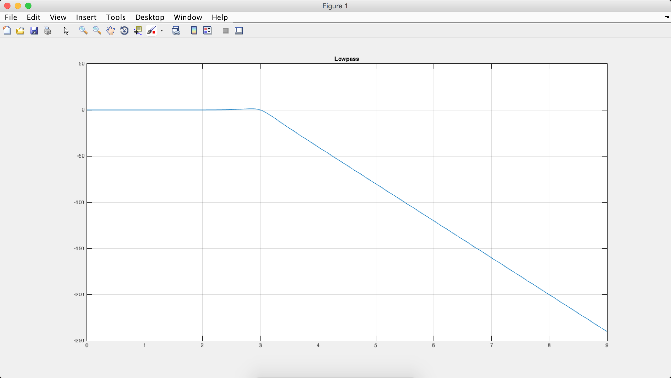
plot(log10(w), 20*log10(abs(t1)));grid on;title('Lowpass') % matlab will now plot our transfer function with respect to the graph we declared 

matlab.zip

Once all of this has been inputted into MATLAB and saved, when the script is run this plot will appear with a low pass with the cutoff at the frequency w0.