
Negative Feedback, Part 1: General Structure and Essential Concepts
This article, the first in a series, will introduce you to the fundamental concepts required for understanding and analyzing negative feedback amplifiers.
This article, the first in a series, will introduce you to the fundamental concepts required for understanding and analyzing negative feedback amplifiers.
Not Just Op-Amps. . .
In this article, we will introduce the general negative feedback structure and the quantities that help us to analyze and implement this structure. More specifically, we will focus on the negative feedback amplifier. The term “amplifier” here is somewhat misleading: this structure is not limited to merely increasing the amplitude of a signal. This “amplifier” could be a unity-gain system that is intended to improve a circuit’s input or output impedance characteristics, or it could be a filter that amplifies certain frequencies while attenuating others.
Why Feedback?
So we have an output variable of some kind that must be controlled, but the relationship between the control input and the actual behavior of the output is so complex or unpredictable that it would be difficult, if not impossible, to precisely regulate the output simply by applying a specified input. Consider two examples: We have a voltage-output digital-to-analog converter (DAC), and we want to control 1) the power dissipated by a resistor and 2) the brightness of an LED. The first task does not require negative feedback because the relationship between input and output is simple and predictable:
\[P\ =\ \frac{V^2}{R},\ \ \ \ V\ =\ \sqrt{PR}\]
All we need to do is multiply the desired power by the resistance and then take the square root. This is fairly simple math for a modern microcontroller, and more importantly, this relationship is valid for any resistor under any environmental conditions. The second task, however, is not so straightforward. Here is a plot of forward current vs. forward voltage for an LED manufactured by Avago:
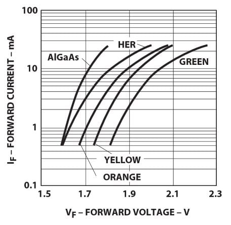
The relationship is highly nonlinear and significantly affected by the type of LED; though not shown in this plot, the relationship is also influenced by temperature. Now take a look at the brightness vs. forward current characteristics:
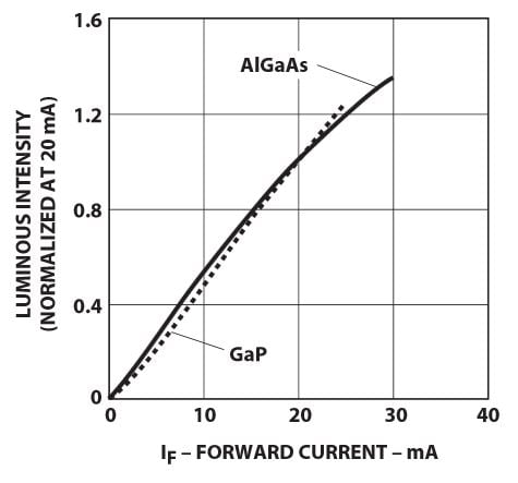
This relationship is quite linear, with minimal difference between the two semiconductor materials. So what do we conclude from this? It would be fairly easy to accurately regulate LED brightness by controlling current, and it would be quite difficult to accurately regulate brightness by controlling voltage. What to do? Bring in some negative feedback, of course! We could use the DAC voltage as the input to a negative feedback amplifier that adjusts its output voltage based on how much current is flowing through the LED (the current information can be measured via a series resistor). Now we have a simple, predictable relationship between voltage and brightness.
This LED example is one of countless situations in which it would be undesirable or completely impractical to implement open-loop (i.e., non-feedback) control. Think about temperature regulation: how could open-loop control possibly account for all the factors that affect the temperate of, say, a living room? Weather conditions, windows, doors, number of occupants. . . . But as demonstrated by the ubiquity of the humble thermostat, with a little negative feedback the problem becomes almost trivial.
The Generic Feedback Amplifier
As you look at this diagram, try to take a minute to appreciate the elegance of negative feedback.
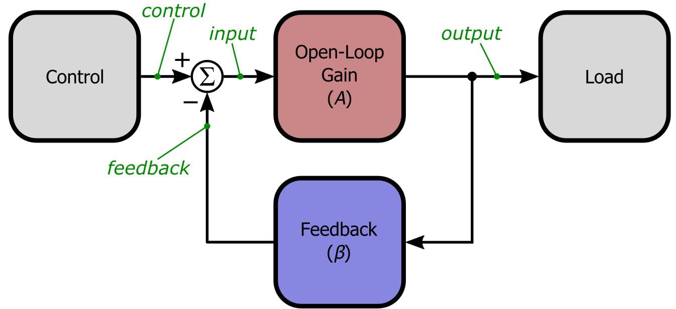
By simply subtracting the actual output value (multiplied by β) from the reference signal and using the result as the input to the open-loop amplifier, we can precisely control the load, even when the input-to-output relationship is inconsistent or complex.
The key parameters here are A and β. The green italicized labels represent variable names for the signals flowing through the system; we are using words (italicized also in the text of this article) instead of subscripted variables in the hope that the forthcoming analysis will not appear less intuitive than it actually is. (We retain A and β, though, because a feedback amplifier is just not a feedback amplifier without A and β.)
So what exactly are A and β? There is not much to say about A: it is the amplification that the overall system would apply in the absence of feedback. In the context of an op-amp circuit—the comparison is particularly apt because the op-amp is such a direct manifestation of the theoretical feedback amplifier—A corresponds to the op-amp’s open-loop gain. β is not quite so straightforward: the feedback factor β determines how much of the output signal is fed back to the subtraction node. You can think of β as the percentage (expressed as a decimal) of output that is subtracted from control. This should become more clear when you think in terms of a basic noninverting op-amp circuit:

The two resistors that we use to set the gain are nothing more than a divider network that applies a certain percentage of the output to the inverting terminal of the op-amp. The voltage across the output resistor is expressed by the ratio R1/(R1 + R2), multiplied by the voltage across the resistor pair. Thus, the percentage (expressed as a decimal) of output fed back and subtracted from control—i.e., the feedback factor β—is R1/(R1 + R2). It is worth your while to cultivate an intuitive understanding of this concept, because β will figure prominently in a future article when we discuss stability.
One more note about A and β: They need not be mere constants, as in A = 106 and β = 0.1. They can also be represented as functions of frequency, meaning that the value of A or β varies according to the frequency of the signal passing through the amplifier system. This is particularly relevant for A—the open-loop gain of internally compensated op-amps starts to roll off at frequencies as low as 0.1 Hz!
Closing the Loop
Now we will briefly cover some salient relationships and formulas that will help us to further understand and analyze the behavior of a feedback amplifier. First is the mathematical definition of β:
\[feedback\ =\ \beta\times output,\ \ \ \ \ \ \beta=\frac{feedback}{output}\]
This is simply a symbolic expression of what we described in the previous section. Next is the straightforward relationship between input and output, readily apparent from the general feedback structure diagram shown above:
\[output\ =\ A\times input\]
Somewhat more interesting is the equation for closed-loop gain (GCL), i.e., the overall gain of the amplifier system when the effect of negative feedback is included.
\[G_{CL}=\frac{output}{control}=\frac{A\times input}{input+feedback}=\frac{A\times input}{input+\left(\beta\times output\right)}=\frac{input\left(A\right)}{input\left(1+\beta\frac{output}{input}\right)}=\frac{A}{1+A\beta}\]
This relationship is pretty simple, but it gets even better. In typical feedback amplifier applications, the quantity Aβ (referred to as the “loop gain”) is much larger than 1—for example, with an open-loop op-amp gain of 106 and a feedback factor of 0.1, the loop gain is 105. Thus, we can simplify the closed-loop gain expression as follows:
\[G_{CL}=\frac{A}{1+A\beta}\approx\frac{A}{A\beta}=\frac{1}{\beta}\]
And here we see exactly what we expect from our experience with op-amp circuits: the gain depends only on β. Look again at the noninverting op-amp circuit shown above; everything comes together when we recall that the gain equation for a standard noninverting amplifier (GNI) is 1 + (R2/R1):
\[G_{NI}=1+\frac{R_2}{R_1},\ \ \ \ \ \ G_{CL}=\frac{1}{\beta}=\frac{R_1+R_2}{R_1}=\frac{R_1}{R_1}+\frac{R_2}{R_1}=1+\frac{R_2}{R_1}\]
Conclusion
After introducing negative feedback and the general motivation for using it, we presented a theoretical model that helps us to analyze the specific characteristics of a negative feedback amplifier. We then employed a little bit of math to demonstrate the most prominent benefit of incorporating negative feedback—namely, for all practical purposes the overall gain of the system is determined completely by the simple (and precise, if necessary) external components that constitute the feedback network. In the next article we will explore some additional ways in which negative feedback can improve the performance of an amplifier circuit.
Next Article in Series: Negative Feedback, Part 2: Improving Gain Sensitivity and Bandwidth


Great! I am looking forward to learning more about ‘feedback’.
I’m thinking that the approach for finding the closed-loop gain is what Mason used to develop his gain formula.
You guys are awesome at explaining things! Keep ‘em coming.