Undesired Effects of a Window Function in FIR Filter Design
A smoother transition band and ripples in the passband are the most important differences between the ideal filters and those designed by window method. This article tries to provide a deeper insight into how truncation leads to these features.
As mentioned in the first part of this article, a smoother transition band and ripples in the passband are the most important differences between the ideal filters and those designed by window method.
This article tries to provide a deeper insight into how truncation leads to these features. The goal of this article is not a mathematically strict and thorough proof— instead, we aim to demonstrate the truncation effects in an intuitive way.
Main Lobe Width and Peak Sidelobe of a Window
Truncation of the impulse response is equivalent to multiplying the desired impulse response, $$h_{d}[n]$$, by a rectangular window, $$w[n]$$. We saw that a time shift in $$h_{d}[n]$$ is necessary to obtain a causal and linear-phase response. Consider the designed filter as
$$h[n]=h_{d}[n-\frac{M-1}{2}]w[n-\frac{M-1}{2}]$$
Equation (1)
where $$w[n]$$ represents a rectangular window which is equal to one for $$n=-\frac{M-1}{2},...,+\frac{M-1}{2}$$ and zero otherwise. Similar to the first part of this article, we will review the concepts using an example. Assume that $$h_{d}[n]$$ is the response of an ideal low-pass filter with cutoff frequency of $$\frac{\pi}{4}$$. Moreover, suppose that $$M$$ is an odd number.
To analyze the frequency response of the designed filter, we need to calculate the discrete-time Fourier transform of Equation (1). From our “Signals and Systems” course, we recall that multiplication in the time domain is equal to convolution in the frequency domain. In order to apply this to Equation (1), we first calculate the spectrum of each term in this equation. Considering the time-shifting property in Fourier transform, we obtain
$$h_{d,new}[n]=h_{d}[n-\frac{M-1}{2}]\overset{F}{\rightarrow}e^{-j\omega \frac{M-1}{2}}H_{d}(\omega)$$
$$w_{new}[n]=w[n-\frac{M-1}{2}]\overset{F}{\rightarrow}e^{-j\omega \frac{M-1}{2}}W(\omega)$$
Equation (2)
where $$H_{d}(\omega)$$ and $$W(\omega)$$ are the Fourier transforms of $$h_{d}[n]$$ and $$w[n]$$, respectively. Hence the Fourier transform of $$h[n]$$ will be
$$H(\omega)=\frac{1}{2\pi}H_{d,new}[\omega]*W_{new}[\omega]=\frac{1}{2\pi} \int_{-\pi}^{+\pi} [e^{-j(\omega-\theta)\frac{M-1}{2}}H_{d}(\omega - \theta))][e^{-j\theta \frac{M-1}{2}}W(\theta)]d\theta$$
Equation (3)
where $$*$$ denotes the convolution. Equation (3) means that we should shift the desired spectrum continuously and multiply the shifted spectrum by the window response and then calculate the integral.
Equation (3) can be simplified as
$$H(\omega)=\frac{1}{2\pi}e^{-j\omega \frac{M-1}{2}} \int_{-\pi}^{+\pi} H_{d}(\omega - \theta) W(\theta) d\theta$$
Equation (4)
It can be easily shown that the spectrum of $$w[n]$$ is
$$W(\omega)=\left\{\begin{matrix} \frac{ sin(\frac{\omega M}{2}) }{sin(\frac{\omega}{2})} & \omega \neq 0\\ M & \omega = 0 \end{matrix}\right \}$$
Equation (5)
The normalized form of this function, $$\frac{W(\omega)}{M}$$, is available in MATLAB through the $$diric(\omega, M)$$ command.
Figure (1) shows $$\frac{W(\omega)}{M}$$ for $$M=21$$.

Figure (1) $$\frac{W(\omega)}{M}$$ for $$M=21$$.
This figure points out the two most important features of a window function, i.e. the “main lobe width” and the “peak sidelobe”. The main lobe width can be calculated by subtracting the first two roots of Equation (5) which are at $$\pm \frac{2\pi}{M}$$. Therefore, the main lobe width of a rectangular window will be $$\frac{4\pi}{M}$$. As shown in Figure (1), the peak sidelobe of a window is the amplitude of the largest sidelobe. We will verify that these two properties determine the smoothness of the transition band and the passband ripples in filters designed by the window method.
Simple Approximations for a Window Spectrum
In order to examine the important features of a window function, we approximate the spectrum in Figure (1) with five triangles as shown in Figure (2).
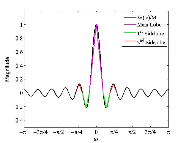
Figure (2) Approximating the window spectrum with 5 triangles.
If we consider $$T_{1}$$, $$T_{2}$$ and $$T_{3}$$ as the equations that, respectively, give the magenta, green, and red triangles of Figure (2), then we obtain
$$\frac{W(\omega)}{M}\approx T_{1} + T_{2} + T_{3}$$
Equation (6)
Notice that each of $$T_{2}$$ and $$T_{3}$$ represent two triangles.
Substituting Equation (6) into Equation (4), we obtain
$$H(\omega)= \frac{1}{2 \pi} e^{-j \omega \frac{M-1}{2}} (H_{d}(\omega) * W(\omega)) \approx \frac{M}{2 \pi} e^{-j \omega \frac{M-1}{2}} (H_{d}(\omega) * (T_{1} + T_{2} + T_{3}))$$
Equation (7)
Due to the distributivity property of convolution, we are allowed to calculate the convolution of $$H_{d}(\omega)$$ with each of $$T_{1}$$, $$T_{2}$$ and $$T_{3}$$, and then add the results to achieve the overall convolution.
The convolution of a rectangular function with a triangle is shown in Figure (3). This figure, actually, demonstrates the convolution of $$T_{1}$$, Figure (3a), with $$H_{d}(\omega)$$, Figure (3b), for $$M=21$$. The convolution result is shown in Figure (3c). Note that the duration of the triangle and $$H_{d}(\omega)$$ is $$\frac{4\pi}{21}$$ and $$\frac{\pi}{2}$$, respectively. However, the duration of the convolution result is $$\frac{4\pi}{21} + \frac{\pi}{2}$$. This is related to a general property of convolution that if two signals, $$x(t)$$ and $$y(t)$$, with durations of respectively $$T_{x}$$ and $$T_{y}$$ are convolved, the duration of the result will be $$T_{x} + T_{y}$$. In our case, this means that if the spectrum of the window was simply a triangle with duration of $$\omega _{1}$$, the transition band of the designed filter would be, roughly, of width $$\omega_{1}$$ too.
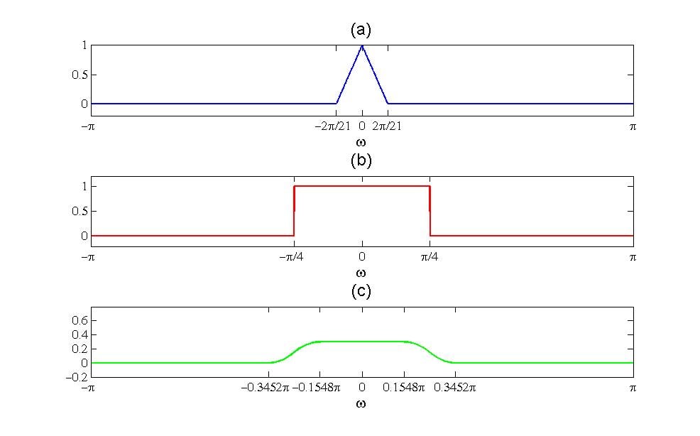
Figure (3) (3a) The normalized triangle approximating the main lobe; (3b) spectrum of the desired filter; (3c) convolution of (3a) and (3b)
Based on the previous discussion, we can easily calculate the convolution of $$H_{d}(\omega)$$ with $$T_{2}$$ and $$T_{3}$$. We only need to take the required x-axis shifts into account and scale the result with respect to the height of each triangle.
Figure (4) shows how $$H_{d}(\omega) * T_{2}$$ is calculated. Figures (4a) and (4b) show the convolution of $$H_{d}(\omega)$$ with the right and left part of $$T_{2}$$, respectively. The shift in the x-axis and the scale in the y-axis correspond to the location and height of the green rectangles in Figure (2). Figure (4c) shows $$H_{d}(\omega) * T_{2}$$ which is the sum of the curves in Figures (4a) and (4b). In a similar manner, $$H_{d}(\omega) * T_{3}$$ can be found. This is shown in Figure (5).
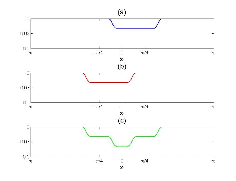
Figure (4) (4a) Convolution of $$H_{d}(\omega)$$ with the right triangle of $$T_{2}$$ ; (4b) convolution of $$H_{d}(\omega)$$ with the left triangle of $$T_{2}$$ ; (4c) convolution of $$H_{d}(\omega)$$ with $$T_{2}$$
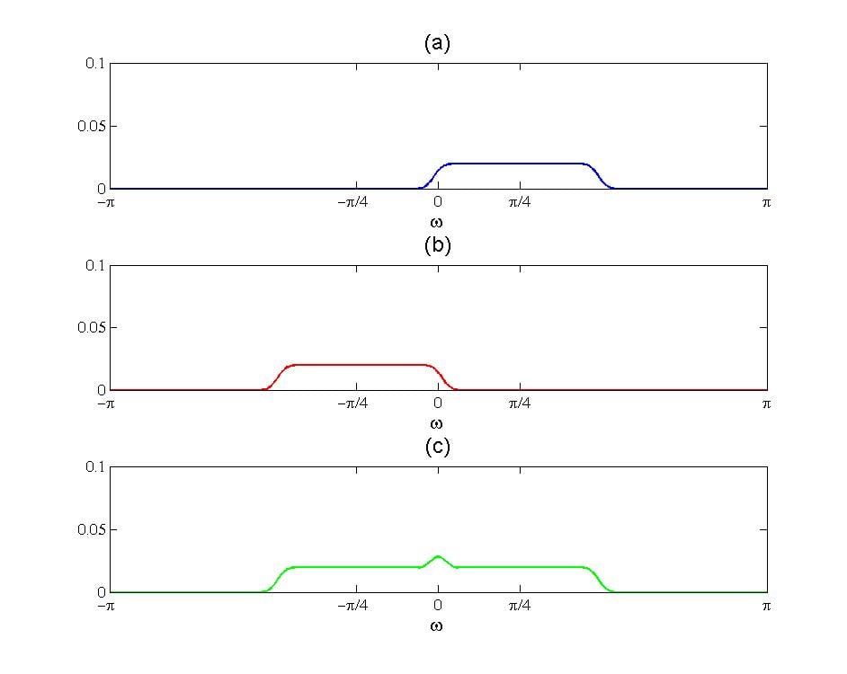
Figure (5) (5a) Convolution of $$H_{d}(\omega)$$ with the right triangle of $$T_{3}$$ ; (4b) convolution of $$H_{d}(\omega)$$ with the left triangle of $$T_{3}$$ ; (4c) convolution of $$H_{d}(\omega)$$ with $$T_{3}$$
Now that we have calculated all the required terms of Equation (7), we can find the response of the designed filter. Figure (6) summarizes the obtained results and shows the sum of them. The most important observations are as follows:
- Please notice that the magnitude of $$H_{d}(\omega) * T_{2}$$ and $$H_{d}(\omega) * T_{3}$$ are much smaller than $$H_{d}(\omega) * T_{1}$$. This is due to the fact that the magnitude of the sidelobes is much smaller than that of the main lobe. Therefore, the overall shape of the frequency response of the designed filter is roughly determined by the main lobe. Approximating the main lobe with a triangle, we saw that the main lobe width increases the transition band. Hence, it is desirable to reduce the main lobe width. For the case of a rectangular window, the main lobe width is equal to $$\frac{4\pi}{M}$$. As a result, in order to achieve a sharper transition, we need to increase the window width, $$M$$.
- Although the overall shape of the designed filter is determined by the main lobe, the sidelobes can produce ripples in the passband and stopband of the achieved filter. The magnitude of the ripples depends on how strong the sidelobes are compared to the main lobe. Usually, the first sidelobe is larger than the other ones. Hence, we can consider the magnitude of the first sidelobe as the parameter which determines the magnitude of ripples in the achieved filter.
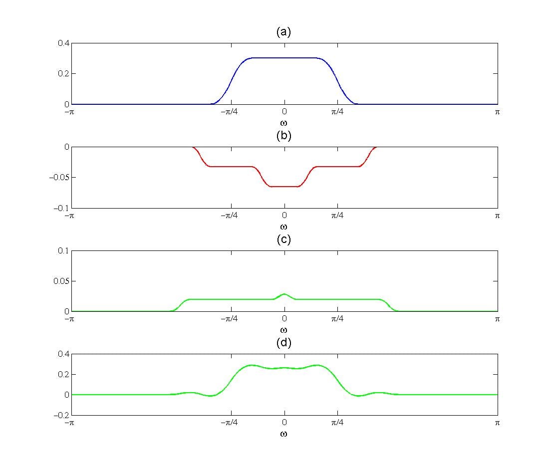
Figure (6) Convolution of $$H_{d}(\omega)$$with (6a) $$T_{1}$$ (6b) $$T_{2}$$ (6c) $$T_{3}$$ and (6d) $$T_{1}+T_{2}+T_{3}$$
Summary
- The spectrum of the rectangular window will make the response of the designed filter deviate from the ideal response.
- The main lobe width affects the transition band of the designed filter.
- To reduce the main lobe width, we may increase the window width, $$M$$. Although this result was shown for a rectangular window, the same conclusion can be drawn for other window functions. Note that, unfortunately, increasing $$M$$ leads to a higher computational complexity. Is there any way, other than increasing $$M$$, to reduce the main lobe width and achieve a sharper transition?
- The peak sidelobe determines the amount of ripples in the passband and stopband of the achieved filter. How can we reduce the peak sidelobe in FIR filter design via window method?