“I think it is safe to say that no one understands quantum mechanics.” —Physicist Richard P. Feynman
To say that the invention of semiconductor devices was a revolution would not be an exaggeration. Not only was this an impressive technological accomplishment, but it paved the way for developments that would indelibly alter modern society. Semiconductor devices made possible miniaturized electronics, including computers, certain types of medical diagnostic and treatment equipment, and popular telecommunication devices, to name a few applications of this technology.
Behind this revolution in technology stands an even greater revolution in general science: the field of quantum physics. Without this leap in understanding the natural world, the development of semiconductor devices (and more advanced electronic devices still under development) would never have been possible. Quantum physics is an incredibly complicated realm of science. This chapter is but a brief overview. When scientists of Feynman’s caliber say that “no one understands [it],” you can be sure it is a complex subject. Without a basic understanding of quantum physics, or at least an understanding of the scientific discoveries that led to its formulation, though, it is impossible to understand how and why semiconductor electronic devices function. Most introductory electronics textbooks I’ve read try to explain semiconductors in terms of “classical” physics, resulting in more confusion than comprehension.
Many of us have seen diagrams of atoms that look something like Figure below.

Rutherford atom: negative electrons orbit a small positive nucleus.
Tiny particles of matter called protons and neutrons make up the center of the atom; electrons orbit like planets around a star. The nucleus carries a positive electrical charge, owing to the presence of protons (the neutrons have no electrical charge whatsoever), while the atom’s balancing negative charge resides in the orbiting electrons. The negative electrons are attracted to the positive protons just as planets are gravitationally attracted by the Sun, yet the orbits are stable because of the electrons’ motion. We owe this popular model of the atom to the work of Ernest Rutherford, who around the year 1911 experimentally determined that atoms’ positive charges were concentrated in a tiny, dense core rather than being spread evenly about the diameter as was proposed by an earlier researcher, J.J. Thompson.
Rutherford’s scattering experiment involves bombarding a thin gold foil with positively charged alpha particles as in Figure below. Young graduate students H. Geiger and E. Marsden experienced unexpected results. A few Alpha particles were deflected at large angles. A few Alpha particles were back-scattering, recoiling at nearly 180o. Most of the particles passed through the gold foil undeflected, indicating that the foil was mostly empty space. The fact that a few alpha particles experienced large deflections indicated the presence of a minuscule positively charged nucleus.

Rutherford scattering: a beam of alpha particles is scattered by a thin gold foil.
Although Rutherford’s atomic model accounted for experimental data better than Thompson’s, it still wasn’t perfect. Further attempts at defining atomic structure were undertaken, and these efforts helped pave the way for the bizarre discoveries of quantum physics. Today our understanding of the atom is quite a bit more complex. Nevertheless, despite the revolution of quantum physics and its contribution to our understanding of atomic structure, Rutherford’s solar-system picture of the atom embedded itself in the popular consciousness to such a degree that it persists in some areas of study even when inappropriate.
Consider this short description of electrons in an atom, taken from a popular electronics textbook:
Orbiting negative electrons are therefore attracted toward the positive nucleus, which leads us to the question of why the electrons do not fly into the atom’s nucleus. The answer is that the orbiting electrons remain in their stable orbit because of two equal but opposite forces. The centrifugal outward force exerted on the electrons because of the orbit counteracts the attractive inward force (centripetal) trying to pull the electrons toward the nucleus because of the unlike charges.
In keeping with the Rutherford model, this author casts the electrons as solid chunks of matter engaged in circular orbits, their inward attraction to the oppositely charged nucleus balanced by their motion. The reference to “centrifugal force” is technically incorrect (even for orbiting planets), but is easily forgiven because of its popular acceptance: in reality, there is no such thing as a force pushing any orbiting body away from its center of orbit. It seems that way because a body’s inertia tends to keep it traveling in a straight line, and since an orbit is a constant deviation (acceleration) from straight-line travel, there is constant inertial opposition to whatever force is attracting the body toward the orbit center (centripetal), be it gravity, electrostatic attraction, or even the tension of a mechanical link.
The real problem with this explanation, however, is the idea of electrons traveling in circular orbits in the first place. It is a verifiable fact that accelerating electric charges emit electromagnetic radiation, and this fact was known even in Rutherford’s time. Since orbiting motion is a form of acceleration (the orbiting object in constant acceleration away from normal, straight-line motion), electrons in an orbiting state should be throwing off radiation like mud from a spinning tire. Electrons accelerated around circular paths in particle accelerators called synchrotrons are known to do this, and the result is called synchrotron radiation. If electrons were losing energy in this way, their orbits would eventually decay, resulting in collisions with the positively charged nucleus. Nevertheless, this doesn’t ordinarily happen within atoms. Indeed, electron “orbits” are remarkably stable over a wide range of conditions.
Furthermore, experiments with “excited” atoms demonstrated that electromagnetic energy emitted by an atom only occurs at certain, definite frequencies. Atoms that are “excited” by outside influences such as light are known to absorb that energy and return it as electromagnetic waves of specific frequencies, like a tuning fork that rings at a fixed pitch no matter how it is struck. When the light emitted by an excited atom is divided into its constituent frequencies (colors) by a prism, distinct lines of color appear in the spectrum, the pattern of spectral lines being unique to that element. This phenomenon is commonly used to identify atomic elements, and even measure the proportions of each element in a compound or chemical mixture. According to Rutherford’s solar-system atomic model (regarding electrons as chunks of matter free to orbit at any radius) and the laws of classical physics, excited atoms should return energy over a virtually limitless range of frequencies rather than a select few. In other words, if Rutherford’s model were correct, there would be no “tuning fork” effect, and the light spectrum emitted by any atom would appear as a continuous band of colors rather than as a few distinct lines.

Bohr hydrogen atom (with orbits drawn to scale) only allows electrons to inhabit discrete orbitals. Electrons falling from n=3,4,5, or 6 to n=2 accounts for Balmer series of spectral lines.
A pioneering researcher by the name of Niels Bohr attempted to improve upon Rutherford’s model after studying in Rutherford’s laboratory for several months in 1912. Trying to harmonize the findings of other physicists (most notably, Max Planck and Albert Einstein), Bohr suggested that each electron had a certain, specific amount of energy, and that their orbits were quantized such that each may occupy certain places around the nucleus, as marbles fixed in circular tracks around the nucleus rather than the free-ranging satellites each were formerly imagined to be. (Figure above) In deference to the laws of electromagnetics and accelerating charges, Bohr alluded to these “orbits” as stationary states to escape the implication that they were in motion. Although Bohr’s ambitious attempt at re-framing the structure of the atom in terms that agreed closer to experimental results was a milestone in physics, it was not complete. His mathematical analysis produced better predictions of experimental events than analyses belonging to previous models, but there were still some unanswered questions about why electrons should behave in such strange ways. The assertion that electrons existed in stationary, quantized states around the nucleus accounted for experimental data better than Rutherford’s model, but he had no idea what would force electrons to manifest those particular states. The answer to that question had to come from another physicist, Louis de Broglie, about a decade later.
De Broglie proposed that electrons, as photons (particles of light) manifested both particle-like and wave-like properties. Building on this proposal, he suggested that an analysis of orbiting electrons from a wave perspective rather than a particle perspective might make more sense of their quantized nature. Indeed, another breakthrough in understanding was reached.

String vibrating at resonant frequency between two fixed points forms standing wave.
The atom according to de Broglie consisted of electrons existing as standing waves, a phenomenon well known to physicists in a variety of forms. As the plucked string of a musical instrument (Figure above) vibrating at a resonant frequency, with “nodes” and “antinodes” at stable positions along its length. De Broglie envisioned electrons around atoms standing as waves bent around a circle as in Figure below.

“Orbiting” electron as standing wave around the nucleus, (a) two cycles per orbit, (b) three cycles per orbit.
Electrons only could exist in certain, definite “orbits” around the nucleus because those were the only distances where the wave ends would match. In any other radius, the wave should destructively interfere with itself and thus cease to exist. De Broglie’s hypothesis gave both mathematical support and a convenient physical analogy to account for the quantized states of electrons within an atom, but his atomic model was still incomplete. Within a few years, though, physicists Werner Heisenberg and Erwin Schrodinger, working independently of each other, built upon de Broglie’s concept of a matter-wave duality to create more mathematically rigorous models of subatomic particles.
This theoretical advance from de Broglie’s primitive standing wave model to Heisenberg’s matrix and Schrodinger’s differential equation models was given the name quantum mechanics, and it introduced a rather shocking characteristic to the world of subatomic particles: the trait of probability, or uncertainty. According to the new quantum theory, it was impossible to determine the exact position and exact momentum of a particle at the same time. The popular explanation of this “uncertainty principle” was that it was a measurement error (i.e. by attempting to precisely measure the position of an electron, you interfere with its momentum and thus cannot know what it was before the position measurement was taken, and vice versa). The startling implication of quantum mechanics is that particles do not actually have precise positions and momenta, but rather balance the two quantities in a such way that their combined uncertainties never diminish below a certain minimum value.
This form of “uncertainty” relationship exists in areas other than quantum mechanics. As discussed in the “Mixed-Frequency AC Signals” chapter in volume II of this book series, there is a mutually exclusive relationship between the certainty of a waveform’s time-domain data and its frequency-domain data. In simple terms, the more precisely we know its constituent frequency(ies), the less precisely we know its amplitude in time, and vice versa. To quote myself:
A waveform of infinite duration (infinite number of cycles) can be analyzed with absolute precision, but the less cycles available to the computer for analysis, the less precise the analysis. . . The fewer times that a wave cycles, the less certain its frequency is. Taking this concept to its logical extreme, a short pulse—a waveform that doesn’t even complete a cycle—actually has no frequency, but rather acts as an infinite range of frequencies. This principle is common to all wave-based phenomena, not just AC voltages and currents.
In order to precisely determine the amplitude of a varying signal, we must sample it over a very narrow span of time. However, doing this limits our view of the wave’s frequency. Conversely, to determine a wave’s frequency with great precision, we must sample it over many cycles, which means we lose view of its amplitude at any given moment. Thus, we cannot simultaneously know the instantaneous amplitude and the overall frequency of any wave with unlimited precision. Stranger yet, this uncertainty is much more than observer imprecision; it resides in the very nature of the wave. It is not as though it would be possible, given the proper technology, to obtain precise measurements of both instantaneous amplitude and frequency at once. Quite literally, a wave cannot have both a precise, instantaneous amplitude, and a precise frequency at the same time.
The minimum uncertainty of a particle’s position and momentum expressed by Heisenberg and Schrodinger has nothing to do with limitation in measurement; rather it is an intrinsic property of the particle’s matter-wave dual nature. Electrons, therefore, do not really exist in their “orbits” as precisely defined bits of matter, or even as precisely defined waveshapes, but rather as “clouds”—the technical term is wavefunction—of probability distribution, as if each electron were “spread” or “smeared” over a range of positions and momenta.
This radical view of electrons as imprecise clouds at first seems to contradict the original principle of quantized electron states: that electrons exist in discrete, defined “orbits” around atomic nuclei. It was, after all, this discovery that led to the formation of quantum theory to explain it. How odd it seems that a theory developed to explain the discrete behavior of electrons ends up declaring that electrons exist as “clouds” rather than as discrete pieces of matter. However, the quantized behavior of electrons does not depend on electrons having definite position and momentum values, but rather on other properties called quantum numbers. In essence, quantum mechanics dispenses with commonly held notions of absolute position and absolute momentum, and replaces them with absolute notions of a sort having no analogue in common experience.
Even though electrons are known to exist in ethereal, “cloud-like” forms of distributed probability rather than as discrete chunks of matter, those “clouds” have other characteristics that are discrete. Any electron in an atom can be described by four numerical measures (the previously mentioned quantum numbers), called the Principal, Angular Momentum, Magnetic, and Spin numbers. The following is a synopsis of each of these numbers’ meanings:
1. Principal Quantum Number
Principal Quantum Number: Symbolized by the letter n, this number describes the shell that an electron resides in. An electron “shell” is a region of space around an atom’s nucleus that electrons are allowed to exist in, corresponding to the stable “standing wave” patterns of de Broglie and Bohr. Electrons may “leap” from shell to shell, but cannot exist between the shell regions. The principal quantum number must be a positive integer (a whole number, greater than or equal to 1). In other words, principle quantum number for an electron cannot be 1/2 or -3. These integer values were not arrived at arbitrarily, but rather through experimental evidence of light spectra: the differing frequencies (colors) of light emitted by excited hydrogen atoms follow a sequence mathematically dependent on specific, integer values as illustrated in Figure previous.
Each shell has the capacity to hold multiple electrons. An analogy for electron shells is the concentric rows of seats of an amphitheater. Just as a person seated in an amphitheater must choose a row to sit in (one cannot sit between rows), electrons must “choose” a particular shell to “sit” in. As in amphitheater rows, the outermost shells hold more electrons than the inner shells. Also, electrons tend to seek the lowest available shell, as people in an amphitheater seek the closest seat to the center stage. The higher the shell number, the greater the energy of the electrons in it.
The maximum number of electrons that any shell may hold is described by the equation 2n2, where “n” is the principal quantum number. Thus, the first shell (n=1) can hold 2 electrons; the second shell (n=2) 8 electrons, and the third shell (n=3) 18 electrons. (Figure below)
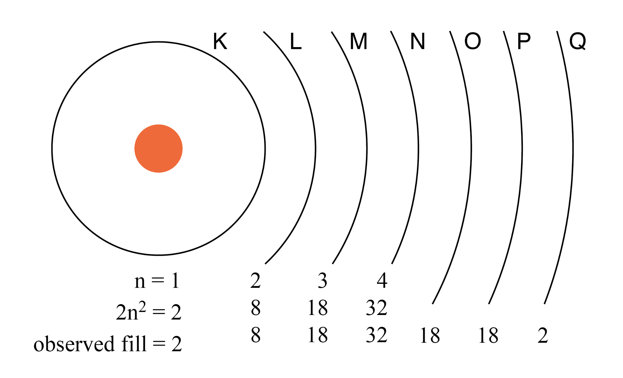
Electron shells in an atom were formerly designated by letter rather than by number. The first shell (n=1) was labeled K, the second shell (n=2) L, the third shell (n=3) M, the fourth shell (n=4) N, the fifth shell (n=5) O, the sixth shell (n=6) P, and the seventh shell (n=7) Q.
2. Angular Momentum Quantum Number
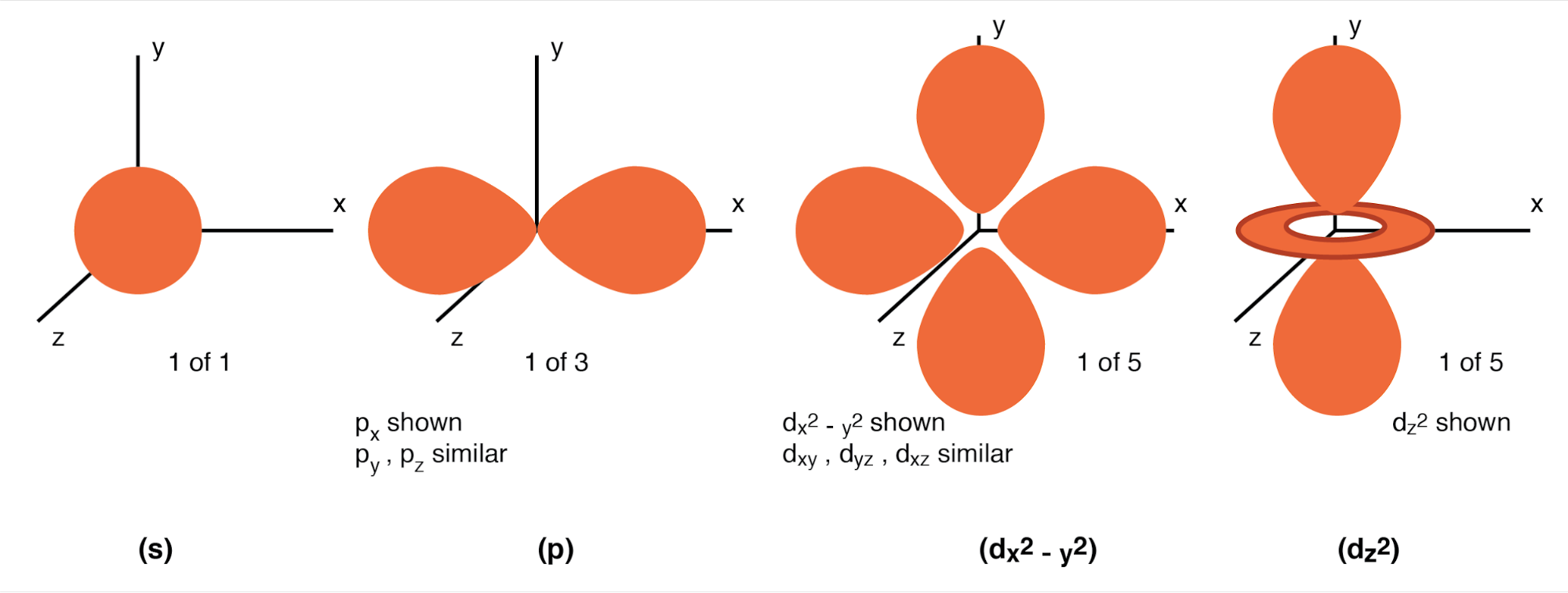
Angular Momentum Quantum Number: A shell, is composed of subshells. One might be inclined to think of subshells as simple subdivisions of shells, as lanes dividing a road. The subshells are much stranger. Subshells are regions of space where electron “clouds” are allowed to exist, and different subshells actually have different shapes. The first subshell is shaped like a sphere, (Figure below(s) ) which makes sense when visualized as a cloud of electrons surrounding the atomic nucleus in three dimensions. The second subshell, however, resembles a dumbbell, comprised of two “lobes” joined together at a single point near the atom’s center. (Figure below(p) ) The third subshell typically resembles a set of four “lobes” clustered around the atom’s nucleus. These subshell shapes are reminiscent of graphical depictions of radio antenna signal strength, with bulbous lobe-shaped regions extending from the antenna in various directions. (Figure below (d) )
Valid angular momentum quantum numbers are positive integers like principal quantum numbers, but also include zero. These quantum numbers for electrons are symbolized by the letter l. The number of subshells in a shell is equal to the shell’s principal quantum number. Thus, the first shell (n=1) has one subshell, numbered 0; the second shell (n=2) has two subshells, numbered 0 and 1; the third shell (n=3) has three subshells, numbered 0, 1, and 2.
An older convention for subshell description used letters rather than numbers. In this notation, the first subshell (l=0) was designated s, the second subshell (l=1) designated p, the third subshell (l=2) designated d, and the fourth subshell (l=3) designated f. The letters come from the words sharp, principal (not to be confused with the principal quantum number, n), diffuse, and fundamental. You will still see this notational convention in many periodic tables, used to designate the electron configuration of the atom's’ outermost, or valence, shells. (Figure below)

(a) Bohr representation of Silver atom, (b) Subshell representation of Ag with division of shells into subshells (angular quantum number l). This diagram implies nothing about the actual position of electrons, but represents energy levels.
3. Magnetic Quantum Number
Magnetic Quantum Number: The magnetic quantum number for an electron classifies which orientation its subshell shape is pointed. The “lobes” for subshells point in multiple directions. These different orientations are called orbitals. For the first subshell (s; l=0), which resembles a sphere pointing in no “direction”, so there is only one orbital. For the second (p; l=1) subshell in each shell, which resembles dumbbells point in three possible directions. Think of three dumbbells intersecting at the origin, each oriented along a different axis in a three-axis coordinate space.
Valid numerical values for this quantum number consist of integers ranging from -l to l, and are symbolized as ml in atomic physics and lz in nuclear physics. To calculate the number of orbitals in any given subshell, double the subshell number and add 1, (2·l + 1). For example, the first subshell (l=0) in any shell contains a single orbital, numbered 0; the second subshell (l=1) in any shell contains three orbitals, numbered -1, 0, and 1; the third subshell (l=2) contains five orbitals, numbered -2, -1, 0, 1, and 2; and so on.
Like principal quantum numbers, the magnetic quantum number arose directly from experimental evidence: The Zeeman effect, the division of spectral lines by exposing an ionized gas to a magnetic field, hence the name “magnetic” quantum number.
4. Spin Quantum Number
Spin Quantum Number: Like the magnetic quantum number, this property of atomic electrons was discovered through experimentation. Close observation of spectral lines revealed that each line was actually a pair of very closely-spaced lines, and this so-called fine structure was hypothesized to result from each electron “spinning” on an axis as if a planet. Electrons with different “spins” would give off slightly different frequencies of light when excited. The name “spin” was assigned to this quantum number. The concept of a spinning electron is now obsolete, being better suited to the (incorrect) view of electrons as discrete chunks of matter rather than as “clouds”; but, the name remains.
Spin quantum numbers are symbolized as ms in atomic physics and sz in nuclear physics. For each orbital in each subshell in each shell, there may be two electrons, one with a spin of +1/2 and the other with a spin of -1/2.
The physicist Wolfgang Pauli developed a principle explaining the ordering of electrons in an atom according to these quantum numbers. His principle, called the Pauli exclusion principle, states that no two electrons in the same atom may occupy the exact same quantum states. That is, each electron in an atom has a unique set of quantum numbers. This limits the number of electrons that may occupy any given orbital, subshell, and shell.
Shown here is the electron arrangement for a hydrogen atom:

With one proton in the nucleus, it takes one electron to electrostatically balance the atom (the proton’s positive electric charge exactly balanced by the electron’s negative electric charge). This one electron resides in the lowest shell (n=1), the first subshell (l=0), in the only orbital (spatial orientation) of that subshell (ml=0), with a spin value of 1/2. A common method of describing this organization is by listing the electrons according to their shells and subshells in a convention called spectroscopic notation. In this notation, the shell number is shown as an integer, the subshell as a letter (s,p,d,f), and the total number of electrons in the subshell (all orbitals, all spins) as a superscript. Thus, hydrogen, with its lone electron residing in the base level, is described as 1s1.
Proceeding to the next atom (in order of atomic number), we have the element helium:

A helium atom has two protons in the nucleus, and this necessitates two electrons to balance the double-positive electric charge. Since two electrons—one with spin=1/2 and the other with spin=-1/2— fit into one orbital, the electron configuration of helium requires no additional subshells or shells to hold the second electron.
However, an atom requiring three or more electrons will require additional subshells to hold all electrons, since only two electrons will fit into the lowest shell (n=1). Consider the next atom in the sequence of increasing atomic numbers, lithium:

An atom of lithium uses a fraction of the L shell’s (n=2) capacity. This shell actually has a total capacity of eight electrons (maximum shell capacity = 2n2 electrons). If we examine the organization of the atom with a completely filled L shell, we will see how all combinations of subshells, orbitals, and spins are occupied by electrons:

Often, when the spectroscopic notation is given for an atom, any shells that are completely filled are omitted, and the unfilled, or the highest-level filled shell, is denoted. For example, the element neon (shown in the previous illustration), which has two completely filled shells, may be spectroscopically described simply as 2p6 rather than 1s22s22p6. Lithium, with its K shell completely filled and a solitary electron in the L shell, may be described simply as 2s1 rather than 1s22s1.
The omission of completely filled, lower-level shells is not just a notational convenience. It also illustrates a basic principle of chemistry: that the chemical behavior of an element is primarily determined by its unfilled shells. Both hydrogen and lithium have a single electron in their outermost shells (1s1 and 2s1, respectively), giving the two elements some similar properties. Both are highly reactive, and reactive in much the same way (bonding to similar elements in similar modes). It matters little that lithium has a completely filled K shell underneath its almost-vacant L shell: the unfilled L shell is the shell that determines its chemical behavior.
Elements having completely filled outer shells are classified as noble, and are distinguished by almost complete non-reactivity with other elements. These elements used to be classified as inert, when it was thought that these were completely unreactive, but are now known to form compounds with other elements under specific conditions.
Since elements with identical electron configurations in their outermost shell(s) exhibit similar chemical properties, Dmitri Mendeleev organized the different elements in a table accordingly. Such a table is known as a periodic table of the elements, and modern tables follow this general form in Figure below.

Periodic table of chemical elements
Dmitri Mendeleev, a Russian chemist, was the first to develop a periodic table of the elements. Although Mendeleev organized his table according to atomic mass rather than atomic number, and produced a table that was not quite as useful as modern periodic tables, his development stands as an excellent example of scientific proof. Seeing the patterns of periodicity (similar chemical properties according to atomic mass), Mendeleev hypothesized that all elements should fit into this ordered scheme. When he discovered “empty” spots in the table, he followed the logic of the existing order and hypothesized the existence of heretofore undiscovered elements. The subsequent discovery of those elements granted scientific legitimacy to Mendeleev’s hypothesis, furthering future discoveries, and leading to the form of the periodic table we use today.
This is how science should work: hypotheses followed to their logical conclusions, and accepted, modified, or rejected as determined by the agreement of experimental data to those conclusions. Any fool may formulate a hypothesis after-the-fact to explain existing experimental data, and many do. What sets a scientific hypothesis apart from post hoc speculation is the prediction of future experimental data yet uncollected, and the possibility of disproof as a result of that data. To boldly follow a hypothesis to its logical conclusion(s) and dare to predict the results of future experiments is not a dogmatic leap of faith, but rather a public test of that hypothesis, open to challenge from anyone able to produce contradictory data. In other words, scientific hypotheses are always “risky” due to the claim to predict the results of experiments not yet conducted, and are therefore susceptible to disproof if the experiments do not turn out as predicted. Thus, if a hypothesis successfully predicts the results of repeated experiments, its falsehood is disproven.
Quantum mechanics, first as a hypothesis and later as a theory, has proven to be extremely successful in predicting experimental results, hence the high degree of scientific confidence placed in it. Many scientists have reason to believe that it is an incomplete theory, though, as its predictions hold true more at micro physical scales than at macroscopic dimensions, but nevertheless it is a tremendously useful theory in explaining and predicting the interactions of particles and atoms.
As you have already seen in this chapter, quantum physics is essential in describing and predicting many different phenomena. In the next section, we will see its significance in the electrical conductivity of solid substances, including semiconductors. Simply put, nothing in chemistry or solid-state physics makes sense within the popular theoretical framework of electrons existing as discrete chunks of matter, whirling around atomic nuclei like miniature satellites. It is when electrons are viewed as “wave functions” existing in definite, discrete states that the regular and periodic behavior of matter can be explained.
REVIEW:
RELATED WORKSHEETS:

In Partnership with Future Electronics
by Jake Hertz


In what order are the sub-shells filled? S,P,D,F. What about the order of filling sub-shell orbitals? Is there a fixed filling pattern?