MEMS Vibration Monitoring: From Acceleration to Velocity
MEMS accelerometers have finally reached a point where they are able to measure vibration on a broad set of machine platforms.
MEMS accelerometers have finally reached a point where they are able to measure vibration on a broad set of machine platforms.
Recent advances in their capability, along with the many advantages that MEMS accelerometers already had over more traditional vibration sensors (size, weight, cost, shock immunity, ease of use), are motivating the use of MEMS accelerometers in an emerging class of condition-based monitoring (CBM) systems. As a result, many CBM system architects, developers, and even their customers are giving consideration to these types of sensors for the first time. Quite often, they are faced with the problem of quickly learning how to evaluate the capability of MEMS accelerometers to measure the most important vibration attributes on their machine platforms.
This might seem difficult at first, as MEMS accelerometer data sheets often express the most important performance attributes in terms that these developers may not familiar with. For example, many are familiar with quantifying vibration in terms of linear velocity (mm/s), while most MEMS accelerometer data sheets express their performance metrics in terms of gravity-referenced acceleration (g). Fortunately, there are some simple techniques for making this translation from acceleration to velocity and for estimating the influence that key accelerometer behaviors (frequency response, measurement range, noise density) will have on important system-level criteria (bandwidth, flatness, peak vibration, resolution).
Basic Vibration Attributes
This process starts with a review of linear vibration from an inertial motion point of view. Within this context, vibration is a mechanical oscillation that has zero mean displacement. For those who don’t want their machines to be moving across the factory floor, zero mean displacement is pretty important! The value of the core sensor in a vibration sensing node will be directly related to how well it can represent the most important attributes of a machine’s vibration. In order to start assessing the capability of a specific MEMS accelerometer in this capacity, it’s important to start with a basic understanding of vibration from an inertial motion point of view.
Figure 1 provides a physical illustration of a vibration motion profile, where the gray box represents the middle point, the blue image represents the peak displacement in one direction, and the red image represents the peak displacement in the other direction. Equation 1 provides a mathematical model that describes the instantaneous acceleration of the rectangular object when it is vibrating at one frequency (fV), at a magnitude of Arms.
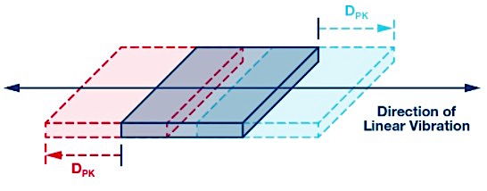
Figure 1. Simple linear vibration motion.
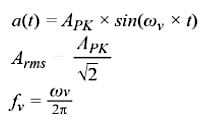
Equation 1
In most CBM applications, the vibration on a machine platform is often going to have more complex spectral signature than the model in Equation 1, but this model provides a nice starting point in the discovery process, as it identifies two common vibration attributes that CBM systems often track: magnitude and frequency. This approach is also useful in translating key behaviors into terms of linear velocity as well (more on that later). Figure 2 provides a spectral view of two different types of vibration profiles. The first profile (see the blue lines in Figure 2) has a constant magnitude across its frequency range, which is between f1 and f6. The second profile (see the green lines in Figure 2) has peaks in its magnitude at four different frequencies: f2, f3, f4, and f5.
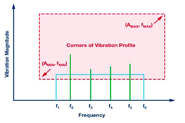
Figure 2. CM vibration profile examples.
System Requirements
Measurement range, frequency range (bandwidth), and resolution are three common attributes that often quantify the capability of a vibration sensing node. The red dashed lines in Figure 2 illustrate these attributes through a rectangular box that is bound by the minimum frequency (fMIN), maximum frequency (fMAX), MIN), maximum frequency (fMAX), minimum magnitude (AMIN), and maximum magnitude (AMAX). When considering a MEMS accelerometer for the role of the core sensor in a vibration sensing node, system architects will likely want to analyze its frequency response, measurement range, and noise behaviors fairly early in their design cycle.
There are simple techniques for evaluating each of these accelerometer behaviors to predict the accelerometer’s suitability for a given set of requirements. Obviously, system architects will eventually need to validate these estimates through actual validation and qualification, but even those efforts will value the expectation that comes from early analysis and predication of the accelerometerʼs capabilities.
Frequency Response
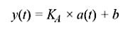
Equation 2 presents a simple, first-order model that describes a MEMS accelerometer’s response (y) to linear acceleration (a) in the time domain. In this relationship, the bias (b) represents the value of the sensor’s output when it is experiencing zero linear vibration (or any type of linear acceleration). The scale factor (KA) represents the amount of change in the MEMS accelerometer’s response (y), with respect to the change in linear acceleration (a).
Equation 2
The frequency response of a sensor describes the value of the scale factor (KA), with respect to frequency. In a MEMS accelerometer, the frequency response has two primary contributors: (1) response of its mechanical structure and (2) the response of the filtering in its signal chain. Equation 3 presents a generic, second-order model that presents an approximation for the mechanical portion of a MEMS accelerometer’s response to frequency. In this model, fO represents the resonant frequency and Q represents the quality factor.
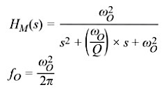
Equation 3
The contribution from the signal chain will often depend on the filtering that the application requires. Some MEMS accelerometers use a single-pole, low-pass filter to help lower the gain of the response at the resonant frequency. Equation 4 offers a generic model for the frequency response associated with this type of filter (HSC). In this type of filter model, the cutoff frequency (fC) represents the frequency at which the magnitude of the output signal is lower than its input signal by a factor of √2.
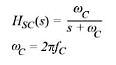
Equation 4
Equation 5 combines the contributions of the mechanical structure (HM) and the signal chain (HSC).
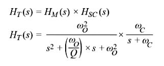
Equation 5
Figure 3 provides a direct application of this model to predict the frequency response of the ADXL356 (x-axis). This model assumes a nominal resonant frequency of 5500 Hz, a Q of 17, and the use of a single-pole, low-pass filter that has a cutoff frequency of 1500 Hz. Note that Equation 5 and Figure 4 only describe the sensor’s response. This model does not include consideration of the manner in which the accelerometer is coupled to the platform that it is monitoring.
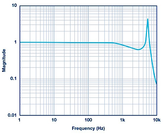
Figure 3. ADXL356 frequency response.
Bandwidth vs. Flatness
In signal chains that leverage a single-pole, low-pass filter (like the one in Equation 4) to establish their frequency response, their bandwidth specification often identifies the frequency at which its output signal is delivering 50% of the power of the input signal. In more complex responses, such as the third-order model from Equation 5 and Figure 3, bandwidth specifications will often come with a corresponding specification for the flatness attribute. The flatness attribute describes the change in the scale factor over the frequency range (bandwidth). Using the ADXL356’s simulation from Figure 3 and Equation 5, the flatness at 1000 Hz is approximately 17% and at 2000 Hz, the flatness is ~40%.
While many applications will need to limit the bandwidth that they can use due to their flatness (accuracy) requirements, there are cases where this may not be as concerning. For example, some applications may be more focused on tracking relative changes over time, rather than absolute accuracy. Another example could come from those who will leverage digital postprocessing techniques to remove the ripple over the frequency ranges that they are most interested in. In these cases, the repeatability and stability of the response is often more important than the flatness of the response over a given frequency range.
Measurement Range
The measurement range metric for a MEMS accelerometer represents the maximum linear acceleration that the sensor can track in its output signal. At some linear acceleration level that is beyond the measurement range rating, the output signal of the sensor will saturate. When this happens it introduces significant distortion and makes it very difficult (if not impossible) to extract useful information from the measurements. Therefore, it is important to make sure that a MEMS accelerometer will support the peak acceleration levels (see AMAX in Figure 2).
Note that the measurement range will have a dependence on frequency since the mechanical response of the sensor introduces some gain to the response, with the peak of the gain response happening at the resonant frequency. In the case of the simulated response for the ADXL356 (see Figure 3), the gain peaks at approximately 4×, which reduces the measurement range from ±40 g to ±10 g. Equation 6 offers an analytical approach to predicting this same number, using Equation 5 as a starting point:
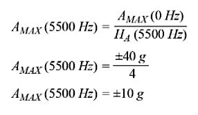
Equation 6
The large change in scale factor and reduction in measurement range are two reasons why most CBM systems will want to confine the maximum frequency of their vibration exposure to levels that are well below the resonant frequency of the sensor.
Resolution
“The resolution of an instrument may be defined as the smallest change in the environment that causes a detectable change in the indication of the instrument.”1 In a vibration sensing node, noise in the acceleration measurement will have a direct influence on its ability to detect changes in vibration (aka “resolution”). Therefore, noise behaviors are an important consideration for those who are considering a MEMS accelerometer to detect small changes in the vibration on their machine platforms. Equation 7 provides a simple relationship for quantifying the impact that a MEMS accelerometer’s noise will have on its ability to resolve small change in vibration. In this model, the sensor’s output signal (yM) is equal to the sum of its noise (aN) and the vibration that it is experiencing (aV). Since there will be no correlation between the noise (aN) and the vibration (aV), the magnitude of the sensor’s output signal (|yM|) will be equal to the root sum square (RSS) combination of the noise magnitude (|aN|) and the vibration’s magnitude (|aV|).
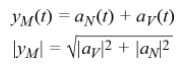
Equation 7
So, what level of vibration is required to overcome the noise burden in the measurement and create an observable response in the sensor’s output signal? Quantifying the vibration level in terms of the noise level can help explore this question in an analytical manner. Equation 8 establishes this relationship through ratio (KVN) and then derives a relationship to predict the level of change in the sensor’s output, in terms of that ratio:
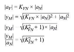
Equation 8
Table 1 provides some numerical examples of this relationship to help illustrate the increase in the sensor’s output measurement, with respect to the ratio (KVN) of the vibration and noise magnitudes. For simplicity, the remainder of this discussion will assume that the total noise in the sensor’s measurement will establish its resolution. From Table 1, this relates to the case where KVN is equal to one, which is when the vibration magnitude is equal to the noise magnitude. When that happens, the magnitude in the sensor’s output will increase by 42% over its output magnitude when there is zero vibration. Note that each application may need to consider what level of increase will be observable in their system in order to establish a relevant definition for resolution in that situation.
| KVN | lyMl/laNl | Increase % |
| 0 | 1 | 0 |
| 0.25 | 1.03 | 3 |
| 0.5 | 1.12 | 12 |
| 1 | 1.41 | 41 |
| 2 | 2.23 | 123 |
Predicting Sensor Noise
Figure 4 presents a simplified signal chain of a vibration sensing node that will use a MEMS accelerometer. In most cases, the low-pass filter provides some support for antialiasing, while the digital processing will provide more defined boundaries in the frequency response. In general, these digital filters will seek to preserve the signal content that represents the real vibration, while minimizing the influence of out of band noise. Therefore, the digital processing will often be the most influential part of the system to consider when estimating the noise bandwidth. This type of processing can come in the form of time-domain techniques, such as a band-pass filter or through spectral techniques, such as the fast Fourier transform (FFT).
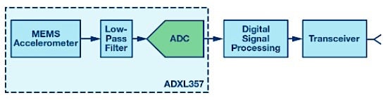
Figure 4. Signal chain of a vibration sensing node.
Equation 9 provides a simple relationship for estimating the total noise in a MEMS accelerometer’s measurement (ANOISE), using its noise density (φND) and the noise bandwidth (fNBW) associated with the signal chain.
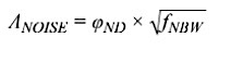
Equation 9
Using the relationship in Equation 9, we can estimate that when using a filter that has a noise bandwidth of 100 Hz on the ADXL357 (noise density = 80 μg/√Hz), total noise will be 0.8 mg (rms).
Vibration in Terms of Velocity
Some CBM applications need to evaluate core accelerometer behaviors (range, bandwidth, noise) in terms of linear velocity. One method for making this translation starts with the simple model from Figure 1 and the same assumptions that produced the model in Equation 1: linear motion, single frequency, and zero mean displacement. Equation 10 expresses this model through a mathematical relationship for the instantaneous velocity (vV) of the object in Figure 1. The magnitude of this velocity, expressed in terms of root mean square (rms), is equal to the peak velocity, divided by the square root of 2.
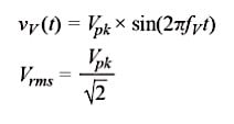
Equation 10
Equation 11 takes the derivative of this relationship to produce a relationship for the instantaneous acceleration of the object in Figure 1:
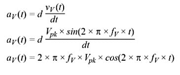
Equation 11
Starting with the peak value of the acceleration model from Equation 11, Equation 12 derives a new formula that relates the acceleration magnitude (Arms) to the velocity magnitude (Vrms) and vibration frequency (fV).
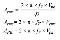
Equation 12
Case Study
Let’s bring this all together with a case study of the ADXL357, which expresses its range (peak) and resolution for a vibration frequency range of 1 Hz to 1000 Hz, in terms of linear velocity. Figure 5 provides graphical definition of several attributes that will contribute to this case study, starting with a plot of the ADXL357’s noise density over the frequency range of 1 Hz to 1000 Hz. For the sake of simplicity in this discussion, all of the computations in this particular case study will assume that the noise density is constant (φND = 80 μg/√Hz) over the entire frequency range. The red spectral plot in Figure 5 represents the spectral response of a band-pass filter and the green vertical line represents the spectral response of a single frequency (fV) vibration, which is useful in developing velocity-based estimates of resolution and range.
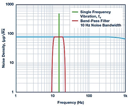
Figure 5. Case study noise density and filtering.
The first step in this process uses Equation 9 to estimate the noise (ANOISE) that comes from four different noise bandwidths (fNBW): 1 Hz, 10 Hz, 100 Hz, and 1000 Hz. Table 2 presents these results in terms of two different units of measure for linear acceleration: g and mm/s2. The use of g is fairly common in most MEMS accelerometer specifications tables, while vibration metrics are not often available in these terms. Fortunately, the relationship between g and mm/s2 is fairly well known and is available in Equation 13.
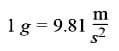
Equation 13
| fNBW(Hz) | ANOISE (mg) | ANOISE (mm/s2) |
|
1 |
0.08 | 0.78 |
| 10 | 0.25 | 2.48 |
| 100 | 0.80 | 7.84 |
| 1000 | 2.5 | 24.8 |
The next step in this case study rearranges the relationship in Equation 12 to derive a simple formula (see Equation 14) for translating the total noise estimates (from Table 2) into terms of linear velocity (VRES, VPEAK). In addition to offering the general form of this relationship, Equation 14 also offers one specific example, using the noise bandwidth of 10 Hz (and the acceleration noise of 2.48 mm/s2, from Table 2). The four dashed lines in Figure 6 represent the velocity resolution for all four noise bandwidths, with respect to the vibration frequency (fV).
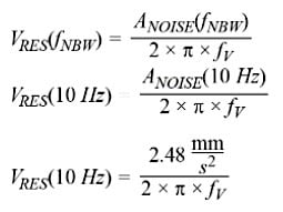
Equation 14
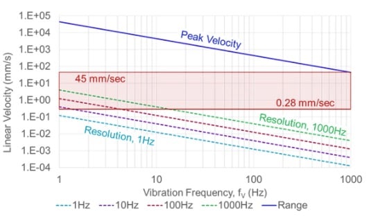
Figure 6. Peak and resolution vs. vibration frequency.
In addition to presenting the resolution for each bandwidth, Figure 6 also provides a solid blue line that represents the peak vibration levels (linear velocity) with respect to frequency. This comes from the relationship in Equation 15, which starts with the same general form as Equation 14, but instead of using the noise in the numerator it uses maximum acceleration that the ADXL357 can support. Note that the √2 factor in the numerator scales this maximum acceleration to reflect the rms level, assuming a single-frequency vibration model.
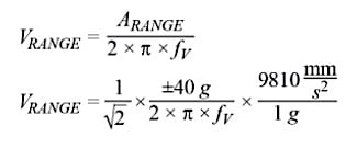
Equation 15
Finally, the red box represents how to apply this information to system-level requirements. The minimum (0.28 mm/s) and maximum (45 mm/s) velocity levels from this red box come from some of the classification levels in a common industry standard for machine vibration: ISO-10816-1. Overlaying the requirements on the range and resolution plots for the ADXL357 provides a quick method for making simple observations, such as:
- The worst case for the measurement range is at the highest frequency, where the ±40 g range of the ADXL357 appears capable of measuring a very large portion of the vibration profiles associated with ISO-10816-1.
- When processing the ADXL357’s output signal with a filter that has a noise bandwidth of 10 Hz filter, the ADXL357 appears capable of resolving the lowest vibration level from ISO-10816-1 (0.28 mm/s) across the frequency range of 1.5 Hz to 1000 Hz.
- When processing the ADXL357’s output signal with a filter that has a noise bandwidth of 1 Hz filter, the ADXL357 appears capable of resolving the lowest vibration level from ISO-10816-1 across the entire 1 Hz to 1000 Hz frequency range.
Conclusion
MEMS accelerometers are coming of age as vibration sensors and they are playing a key role in what appears to be a perfect storm of technology convergence in CBM systems for modern factories. New solutions in sensing, connectivity, storage, analytics, and security are all coming together to provide factory managers with a fully integrated system of vibration observation and process feedback control. While it is easy to get lost in the excitement of all of this amazing technology advancement, someone still needs to understand how to relate these sensor measurements to real-world conditions and the implications that they represent. CBM developers and their customers will be able to draw value from these simple techniques and insights, which provide an approach for translating MEMS performance specifications into their impact on key system-level criteria using familiar units of measure.
References
Gerald C. Gill and Paul L. Hexter. “IEEE Transactions on Geoscience Electronics.” IEEE, Vol. 11, Issue. 2, April 1973.
Industry Articles are a form of content that allows industry partners to share useful news, messages, and technology with All About Circuits readers in a way editorial content is not well suited to. All Industry Articles are subject to strict editorial guidelines with the intention of offering readers useful news, technical expertise, or stories. The viewpoints and opinions expressed in Industry Articles are those of the partner and not necessarily those of All About Circuits or its writers.