Packing More Brains Into Buds: Multi-Feature AI on Tiny Silicon

Earbuds and hearing aids are quietly turning into pocketable computers. On any given day they’re expected to clean up calls, pull a wake word out of a noisy café, understand a short command, and more recently, help follow a friend’s voice at a crowded table. Product teams want to ship all of that without a bigger battery or pricier silicon.

The trick isn’t one magic model or a faster core. It’s a stack of compression techniques: sparsity, quantization, and memory-aware scheduling. Together, they let several small models coexist and cooperate in real time.

Figure 1. Wireless earbuds continue to evolve with new features and capabilities.

Product managers, executives and engineers need practical ways to think about that stack, grounded in real numbers from audio wearables. These tips will allow them to bring more value to their devices without blowing up the BOM or power budget.

The Constraint Box: What Has to Fit

Modern hearables are converging: True Wireless Stereo (TWS) earbuds add assistive listening features; hearing aids add connectivity and richer UX, and premium headsets inch toward health and fitness. Typical “wish lists” now include:

Real-time speech enhancement for calls and for face-to-face denoising (cocktail-party scenarios).

• Wakeword + spoken language understanding (SLU) + voice ID for hands-free control and personalization.
• Feedback cancellation, adaptive EQ compression/ANC
• Biotracking/activity (PPG/optical temperature sensor)
• Activity tracking (IMU/accelerometer)

Design realities: end-to-end audio latencies of 4–10 ms, always-listening features that must idle in microwatts, tight on-chip SRAM, and fixed flash footprints. You can’t meet those constraints with a single technique; you need multiple, complementary ones.

Compression is Plural: The Stack That Actually Fits

Quantization. Moving from float32 to INT8 weights yields an immediate 4× storage reduction and energy savings from narrower datapaths. Many audio models tolerate INT8 with minimal quality impact when per-channel scales are used. Quantization aware training helps further narrow the gap between quantized and float performance, converging to near pre-quantized accuracy within a few additional training steps.

Weight sparsity. Pruning 90% of weights provides roughly 10× smaller parameter storage (which also cuts SRAM leakage), and when the hardware actually skips zero weights (vs. decompressing the weight matrices to do the matrix-vector operation), it provides about 10× fewer MACs in the pruned layers. Importantly, sparsity should be a first-class citizen in the compiler and hardware; otherwise, you pay index/packing overheads without the runtime wins.

Activation sparsity. Speech is bursty. Even without special activation sparsity incentivizing losses, we routinely observe ~50%-70% sparse activations in streaming audio models (more in a quieter environment), in other words, a 2×–3.33× runtime MAC reduction when the hardware can skip zeros on the fly. Utilizing one of the most popular activation functions for artificial neural networks, the rectified linear unit (ReLU), throughout the network yields these zero outputs, which get propagated through the rest of the network. Multiplying or adding by zero yields trivial results at each output layer. Instruction sets that actively look for and skip zero activations dynamically are key to exploiting this observation.

Multiplicative benefits. Weight and activation sparsity are largely uncorrelated, so their runtime effects multiply. A 10× weight-sparsity MAC reduction combined with a 3.3× activation-sparsity reduction is roughly 33× fewer effective operations; before accounting for INT8 efficiency. That’s where the headroom for additional models comes from, both in storage and in saved throughput.

Architecture and memory shaping. Distill to smaller students; use causal temporal convolutional networks (TCN) or tiny-state recurrent neural networks (RNN) models for low-latency streaming; fuse operators to reduce pass-throughs of SRAM; take advantage of activation reuse; tile with the memory hierarchy in mind, and configure sparsity patterns to improve lookup overhead and speedup - just don’t make it so restrictive as to limit the expressivity of the matrices and inhibit performance. For multi-feature systems, share frontends (STFT/delta-LMFB) so features don’t recompute the same buffers.

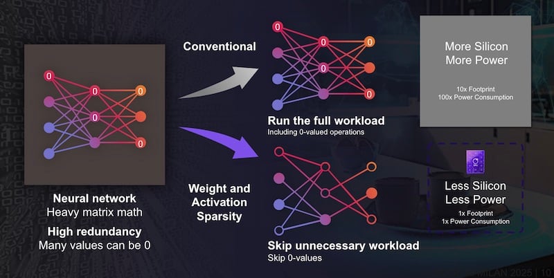
Figure 2. Visual representation of weight and activation sparsity in a simple feedforward neural network. The nodes represent activations in the network, and the connections between nodes represent the weights. Skipping operations on zero values for the nodes and reducing the number of connections between nodes represent activation and weight sparsity, respectively.

A Concrete Example of the Earbud Stack

Consider a real-time temporal convolutional recurrent neural network (TCRNN) speech-enhancement model. This model is nearly 30 layers and too large for most hardware platforms without external DRAM to shuffle weights on and off during runtime. Dense, it has ~6 M parameters or about 24 MB in float precision. With INT8, it drops to ~6 MB. With 90% weight sparsity, it’s ~600 kB for weights; add ~100 kB for activation buffers (≈700 kB total with reuse). Subjectively and objectively, it performs like a much larger model but with a fraction of the footprint.

That footprint is small enough to coexist with other features. For instance, in a 1 MB SRAM footprint, you can reserve ~300 kB for a wake word + SLU path (for example, compress a ~500 kB baseline into ~100 kB with modest sparsity and INT8) and still leave ~200 kB for voice-ID embeddings, sound event detectors, feedback cancellers, or IMU activity classifying models.

In addition to offering more applications per unit silicon, power and latency are where sparsity really shines: the denoiser runs at 8 ms latency for ~1.2 mW, or 4 ms for ~2.1 mW. On a 100 mAh cell, that keeps plenty of budget for radios as well as the other features and their sensors, especially for “situational use” modes or heavily duty cycled workloads.

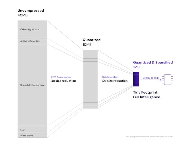
Figure 3. Compression of an earbud AI application stack. 90% sparsity enables a 10x reduced memory footprint with little to no drop in accuracy or performance.

Sharing (and Scheduling) is Caring: Useful Tips

Even perfectly compressed models can waste power if they all run all the time. A practical pattern for earbuds and hearing aids is gated scheduling. Consider these steps:

1. Keep an ultra-low-power listener (wake word, transient/voice activity) on at all times. This is the smallest, least power-hungry model (~200 microwatts including frontend)
2. When it triggers, spin up heavier tasks (SLU, context updates) only as needed, then spin them down into SRAM retention mode.
3. Share features and unify frontends. The denoiser’s acoustic features can also feed environment classification or voice ID. Take the highest resolution FFT you need out of every application (likely speech enhancement or stem splitting) and fuse FFT bins for lower complexity tasks to avoid recomputing frontends. This will help avoid death by buffers
4. Keep any tokenizers or embeddings tiny; cache per-user voiceprints, and use low-rank adapters for personalization instead of whole-model forks.
5. For bio and activity tracking, lean on compact temporal models (TCNs/RNNs) that quantize well; downsample and compress time windows aggressively. Duty cycle when you are sampling at all (heart rate and temperature don’t need to be tracked 24/7); ramp up sampling when large deltas occur or when the user opens a paired health/fitness application for higher accuracy. Activity classifiers often live happily under 100–200 kB with INT8 and modest sparsity.
6. Use ring buffers for streaming and reuse activation/state buffers across tasks to avoid SRAM fragmentation.

Activation sparsity helps here too. On voiced segments, activation density rises and falls with speech; the accelerator naturally does less work when there is less work to be done.

What to Look for in Silicon

If you’re evaluating compute for a multi-feature audio device, check for:

• First-class weight and activation sparsity. It isn’t enough to store sparse weights; you want hardware that skips zero weights and zero activations without extra unpacking or overhead.
• Mixed precision. Efficient INT8 (and increasingly, INT4) for most layers, INT8/16 for activations. Virtualized higher bitwidth precision (combining an INT16 and INT8 operation to form a 24-bit) as an escape hatch for sensitive layers like frontends is a great bonus that reduces the load on accompanying DSPs.
• On-chip memory that matches your concurrency plan. Enough SRAM to hold the denoiser plus a listener plus a small SLU, and ping-pong buffers, without thrashing external memory.
• Streaming-friendly and fused operators. Causal convolutions, small-state RNN cells, future-proof custom operator support for emerging networks like SSMs and sliding-windowed attention, burst-friendly DMA, and multiple power cycling modes.
• A sparsity-aware toolchain. Consider pruning, calibration, packing, and a profiler that reports effective MACs (post-sparsity), not just theoretical GOPs.

You can buy purpose-built sparse accelerators such as these today. The SPU-001 processor from FemtoAI, for example, has 1 MB of SRAM or 10 MB of effective memory at 90% sparsity. It’s 3.4 mm² on the sweetspot node of 22 nm. It supports the techniques mentioned above and treats sparsity as a first-class citizen.

The company has already created most of the AI application stack for their customers. Of course, you could compose a similar sparse earbud application stack, toolchain, compiler, and instruction set, using a general NPU IP with many tiresome, head-scratching engineering hours. Either way, the wins show up only if sparsity is end-to-end: training to packing to runtime.

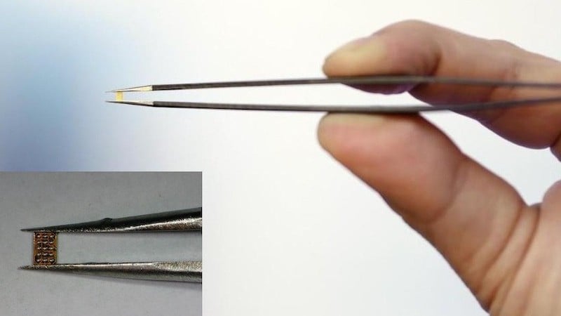
Figure 4. femtoAI’s SPU-001 chip

Quick Planning Checklist Before You Spec Silicon

• List simultaneous features and their worst-case overlap (for example, denoise + wake + SLU + radio).
• Set latency budgets per path (for example, ≤10 ms for denoise; ≤32ms SLU).
• Choose targets for quantization and pruning (for example, INT8 weights everywhere; INT16 for most activations and virtual INT24 when needed, 80–90% sparsity where it's stable).
• Plan to save model checkpoints along different levels of sparsity to have a curve from which to select a performance vs. compression point.
• Verify activation sparsity on your real audio; assume ~50% attainable without special losses.
• Measure with objective metrics (SNR/STOI/PESQ/HASPI/HASQI/DNSMOS for speech; F1 score and FAR/FRR for wakeword/ID) before and after compression.
• Tune detection thresholds with compression along the model checkpoint curve to meet performance requirements.
• Run an early burn-in at the board level with sensors, radio, host processor, speakers, and worst-case number of models running concurrently in a given user scenario; log effective MACs and estimate thermals

Closing: The Multipurpose Future

The market direction is clear: hearables will serve as assistants, communicators, hearing aids, and health companions. To ship that breadth on tiny batteries and tight BOMs, treat compression as a system design discipline, not an afterthought. Quantization gives you the first 4×. Weight sparsity adds ~10×.

Activation sparsity multiplies another ~2–3.3× at runtime. Together, combined with sensible scheduling and shared frontends/features, these gains translate into more applications per microwatt, millimeter, and dollar, or improved performance for a given pre-sparsity budget.

Whether you adopt a sparsity-first accelerator and toolkit like SPU-001 or assemble the stack yourself, the principle is the same: compression isn’t about one model looking clever in isolation; it’s how many models cooperate in the same budget to make the device meaningfully better for the user.

Figure 1 used courtesy of Adobe Stock (licensed)

All other images used courtesy of femtoAI.