Facebook
 Google
 GitHub
 Linkedin
Industry White Paper
Fixed Logic, Software, or eFPGA? Partitioning DSP in Hybrid SoCs
A vector CPU can match an FPGA’s throughput for a 64-tap FIR filter, but it consumes several times the energy per sample. Here’s a practical framework for deciding which signal-processing functions to harden, which to run in software, and which to keep reconfigurable using an embedded FPGA (eFPGA).
Key Takeaways:
- Programmable logic beats software-programmable solutions on energy, not clock speed. In the FIR example below, it uses about 10–17 nJ per sample versus 20–67 nJ for a vector CPU.
- Harden what will never change. Reserve eFPGA for the 10–20% of the DSP workload most likely to evolve.
- Know the cost. eFPGA has 5–10× lower logic density and 2–3× higher power per operation than fixed logic, but updating algorithms after tape-out costs far less than taping out a new ASIC.
Every ASIC tape-out is a bet that the algorithms you harden today will still be the right ones years from now. In signal processing, that bet keeps getting harder to win. Modulation schemes, filter banks, and beamforming modes evolve long after the mask set is paid for, and multi-standard platforms must support several at once.
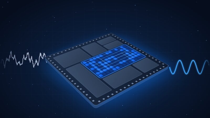
That leaves SoC architects with a familiar tradeoff. Fixed logic delivers unmatched throughput and efficiency, but it can’t change after tape-out. Software-programmable processors are flexible, but they often miss hard real-time constraints and consume more power.
What Is an eFPGA, and How Does It Enable Hybrid Signal Processing?
An embedded FPGA (eFPGA) is reconfigurable logic fabric, the same kind used in FPGA chips, licensed as IP and built directly into an SoC or ASIC. In a hybrid signal-processing design, it sits alongside CPUs, vector processors, DSP cores, and fixed accelerators and runs the functions most likely to change, so you can update them after tape-out without a silicon re-spin.
A hybrid approach with eFPGA offers:
- 10–100× acceleration of critical kernels, such as correlation and matrix multiplication, compared with running them in software
- Lower power than a vector processor for MAC-intensive filters
- Better power and area efficiency than a standalone FPGA chip, because redundant I/O, logic, SerDes, and PHYs are eliminated
- Dynamic reconfiguration to switch processing modes on demand for different protocols, sensor types, or waveform profiles
How Does Programmable Logic Compare With a Vector CPU for DSP?
In modern signal-processing workloads, sustained throughput and energy efficiency matter more than peak clock frequency. A high-performance vector processor can run DSP algorithms efficiently, but it’s still a sequential machine that reuses its arithmetic hardware across operations. Programmable logic implements the algorithm directly in hardware, so operations happen simultaneously and with deterministic timing.
The payoff isn’t just speed. It’s the ability to sustain high data rates inside a tight power envelope, a key requirement in communications, radar, and edge-AI sensing. Table 1 shows how a high-speed, 64-tap FIR filter maps onto each architecture.
Table 1. Implementing a 64-tap FIR filter on a vector CPU versus programmable logic. The FPGA column uses a discrete device as a reference point.
| Criteria 64-tap FIR filter |
Vector CPU e.g., Arm® SVE |
FPGA e.g., AMD (Xilinx) UltraScale™+ |
| Processing style | Sequential vector processing (SIMD) | Spatial parallel processing |
| Parallelism | ~16–32 lanes per SIMD instruction | All filter taps compute simultaneously |
| Arithmetic resources | Limited ALUs reused across operations | Dedicated multiplier per tap (64 multipliers) |
| Pipeline behavior | MAC operations serialized across cycles | Fully pipelined datapath |
| Cycles per sample | ~4–6 (pipeline + memory-fetch latency) | 1 sample per clock |
| Memory access | Depends on cache and memory bandwidth | Data streams directly through the fabric |
| Determinism | Affected by cache misses and OS scheduling | Fully deterministic timing |
| Clock frequency | ~2 GHz | ~300 MHz |
| Achievable sample rate | ~300–500 MS/s (heavily optimized) | ~300 MS/s sustained |
| Power | ~10–20 W (high-performance core) | ~3–5 W |
| Energy per sample* | ~20–67 nJ | ~10–17 nJ |
*Calculated from the sample-rate and power rows above. Figures are representative estimates, not benchmarks.
Look at the bottom rows. The two architectures reach similar sample rates, but the FPGA does it at about one-seventh the clock frequency and a fraction of the power. Per sample, that works out to as much as 6× less energy.
Processors aren’t unsuitable for DSP. But once sustained throughput and power efficiency become system-level constraints, spatial architectures such as programmable logic become the practical choice. That’s exactly the class of workload where embedded programmable logic earns its place in an SoC: an eFPGA implements the same spatial datapath without a standalone FPGA’s package, I/O, and SerDes overhead.
What Does a Hybrid eFPGA SoC Look Like?
A hybrid approach uses fixed logic for known, stable functions and eFPGA for functions that may change, whether to serve different end applications or to add new capabilities such as waveform types, filter banks, or adaptive beamforming modes. In a representative SoC (Figure 1):
- The software-programmable CPU/DSP handles control, adaptation, and lower-ratecomputation.
- Fixed logic (ASIC DSP or hardware accelerators) implements deterministic pipelines that are always required, such as FFT or channelization.
- eFPGA fabric bridges the gap, implementing reconfigurable kernels or extensions that may change over time.
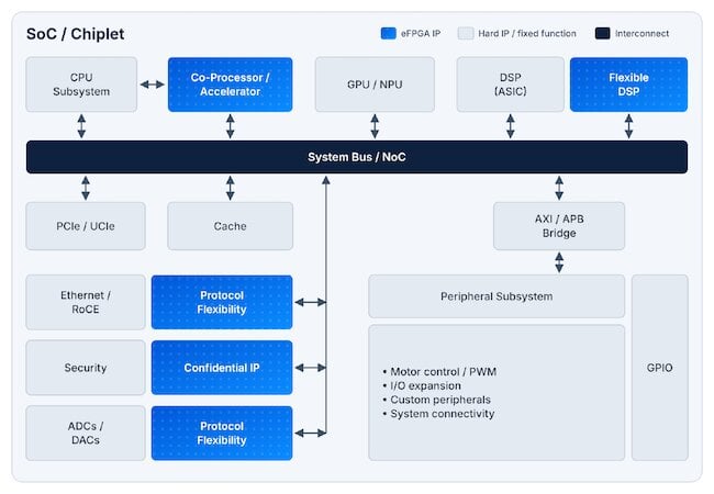
Figure 1. A representative SoC/chiplet architecture. eFPGA blocks (blue) sit beside hard IP to add a flexible co-processor, a flexible DSP, protocol flexibility on high-speed and data-converter interfaces, and a place to load confidential IP after fabrication. Image used courtesy of QuickLogic.
How Do You Decide What Goes in eFPGA vs. Fixed Logic?
It depends on the target markets, systems, and applications, as well as the ASIC's intended lifespan. Table 2 offers general guidelines.
Table 2. General guidelines for partitioning functions between fixed logic and eFPGA.
| Criteria | Use fixed logic when… | Use eFPGA when… |
| Algorithm stability | The function will always be needed (e.g., a fixed FIR filter) | You need to support a range of future algorithms |
| Latency | Hard real-time (< 100 ns) | Near real-time with pipelined RTL |
| Power efficiency | Ultra-low power is required | Very low power is acceptable (using eHVT standard cells) |
| Bit width | Fixed and well defined | Variable precision from multiple data sources |
| Hardware updates | None expected | Anytime during the product lifetime |
Consider a 5G/6G modem or a phased-array radar SoC. FFT and DUC/DDC chains are base filtering functions that will almost always be required, so they belong in fixed accelerators. Adaptive beamforming, pulse compression, and digital filters are different. They may need updates to address new spectral bands, new beamforming coefficients or array geometries, or changes to modulation and coding schemes. Those are eFPGA candidates.
What Are the Area, Power, and I/O Tradeoffs of eFPGA?
eFPGA adds flexibility, but it isn’t free. Plan for these implications:
- I/O: There’s no external I/O overhead, but the fabric still needs ports to on-chip buses, SerDes, and data converters. A high port count can force a larger fabric than the planned logic alone requires.
- Area: Logic density is typically 5–10× lower than standard-cell ASIC logic. That’s acceptable for the small portion of the design that needs reconfigurability.
- Power: Power per operation is roughly 2–3× higher than fixed logic, but it can be up to 10× lower than a discrete FPGA or a software implementation.
Rule of thumb: Put 10–20% of the design’s total DSP workload in eFPGA, the portion that benefits most from hardware adaptability.
Example: How Would You Partition a Wideband Digital Receiver?
Figure 2 shows one way to split a wideband digital receiver pipeline:
- Front-end ADC interface → hard logic
- Polyphase filter bank → fixed accelerator
- Adaptive equalization/beamforming → eFPGA, for algorithm agility
- Control and mode selection → CPU/DSP
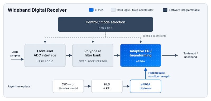
Figure 2. Partitioning a wideband digital receiver. When requirements change, a new bitstream updates the eFPGA stage in the field while the hardened stages stay untouched. Image used courtesy of QuickLogic.
When requirements shift, such as a new modulation scheme or adaptive spatial filtering, you only update the eFPGA bitstream. No silicon re-spin is required. High-level synthesis and model-based design tools, such as Rise Design Automation, Siemens Catapult™ HLS, and MathWorks HDL Coder™, can generate new RTL from C/C++ or Simulink® models. The eFPGA programming tools then compile that RTL into a bitstream.
Design for the Algorithms You Haven’t Written Yet
The silicon you tape out this year will likely ship in systems running algorithms that don’t exist yet. A hybrid architecture lets you plan for that instead of guessing. Start by listing the functions you’re confident will never change, and harden them. Everything else- the adaptive filters, beamformers, and protocol handlers most likely to evolve- is a candidate for eFPGA fabric.
Done right, that partition gives you:
- Post-silicon algorithm updates
- Faster adaptation to evolving standards
- Acceleration of select DSP functions without a full hardware redesign
In effect, eFPGA turns a static ASIC into a reconfigurable compute platform, with fixed-function efficiency where you need it and programmability where you’ll want it.
Sizing a fabric for your next SoC? Explore QuickLogic eFPGA IP and the Australis™ eFPGA IP Generator.