What You Need to Know About EMC Losses

Need a quick refresher on some EMC and EMI basics first? Check out this article before diving in.

 

EMC Loss & Complex Permeability: µ’ vs. µ”

The reality of life and electronics is that everything has losses. The key is to understand what your losses are and how you can control them as best as possible.

 

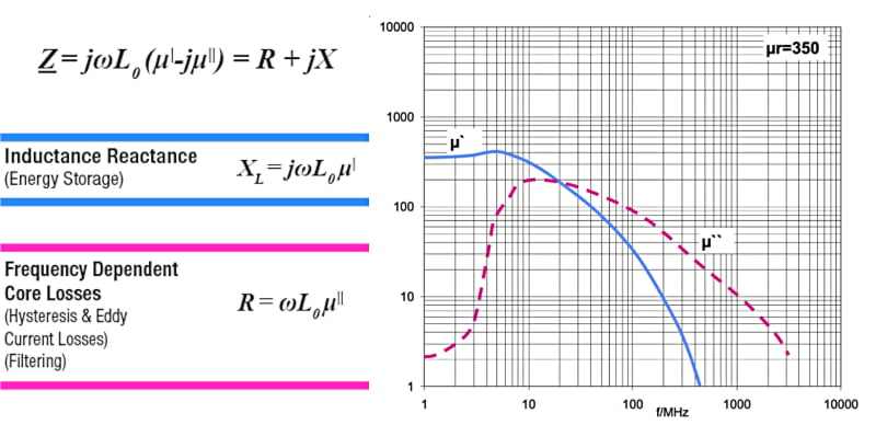
Figure 1. Electromagnetic Core Manufacturers usually specify two important values for the material used to produce the core of an electromagnetic component: µ’ & µ”.

 

µ' represents the inductive reactance of a material and shows the frequency range where it is best used as an inductor. In this image, µ' is the blue line.

µ” represents the losses of the material (resistivity) where the part is best used as a resistor (represented by the pink line). 

The same component can be used for filtering in two different ways, both frequency dependent. Below the cross over frequency, it can be used as a low loss inductor whose impedance diverts currents to ground through capacitors as in LC filters. Above the cross over frequency, it can be used as a lossy resistor used to convert high frequency currents into to heat, thereby eliminating them.

 

The Best Material for Different Frequencies

Different materials have different frequency responses. Here, we're providing you with guidelines for what materials are best suited for what frequencies. Keep in mind that this is just a guide based on a typical situation; as with anything else, there are always exceptions.

 

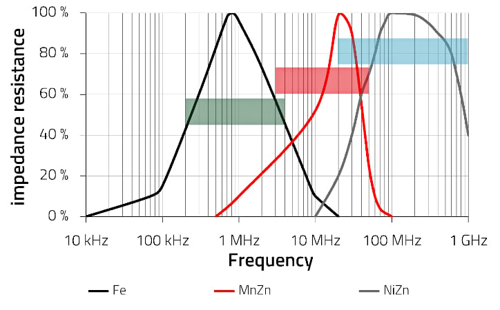
Figure 2. Performance of different materials at different frequencies.

 

• Iron powder (Fe): Typically used for lower frequencies for noise attenuation because it has the highest core losses at frequencies between 200 kHz to 4 MHz. (Shown in black)
• Manganese zinc (MnZn): Typically used for frequencies between 3 MHz and 60 MHz. (Shown in red)
• Nickel zinc: (NiZn): Typically used at frequencies between 20 MHz to 2 GHz because it's very resistive at higher frequencies. (Shown in grey)

 

Insertion Loss Calculation

In the previous section, we have discussed complex permeability and different core materials. This section will cover an important parameter for EMC, which is an insertion loss. The insertion loss is defined as the amount of energy (power) lost by inserting the component into the signal path. It is highly dependent on factors such as path length and core material. The reduction of signal strength is also called attenuation, which is directly proportional to length of the conductive path. If you enjoy performing long mathematical equations, you’ll love this next part. If you don't, you may love it even more! That’s because we have some tips and tricks to help you save both time and energy spent on mathematical equations and using some of our models.

 

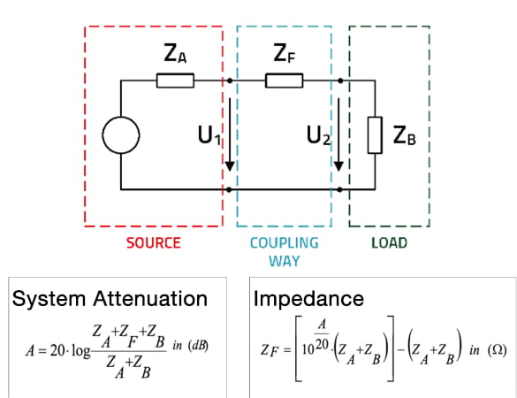
Figure 3. Formulas for calculating insertion loss.

 

As you can see in Figure 3, there are elaborate calculations for system attenuation (A) and impedance (ZF) that determine how much you need for a component to be within a specific attenuation. Because of the parasitic properties of the component, it becomes very difficult and time-consuming to get the mathematics right.

 

Calculating the System Impedance and Using a Nomogram

If you have time and are up to the mathematical challenge, feel free to use the equations above. However, if you want an easier way, we will walk you through how to use this nomogram. 

 

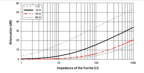
Figure 4. Nomogram for determining the necessary filter impedance.

 

Let’s first take a look at the application overview table. It provides a list of possible applications alongside the assumed practical system impedance, which gives you an idea of the impedance of the whole system for that application.

 

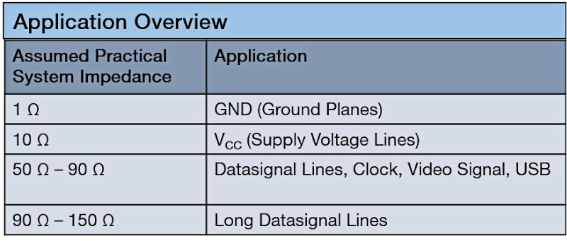
Figure 5. Legend for determining assumed practical system impedance based on application.

 

How do you know what type of application to use? First, you can look at your schematic or board.  In Figure 6, you can see the ground plane, supply voltage line, and data signal line. 

If it is not obvious from the bottom of your board, you can look at the top of the board. With a quick glance you should be able to identify the connectors, power plug, and power lines. 

Once you know the application, you’ll be able to look back at the application overview table to find the assumed practical system impedance you’ll need for using the nomogram. 

 

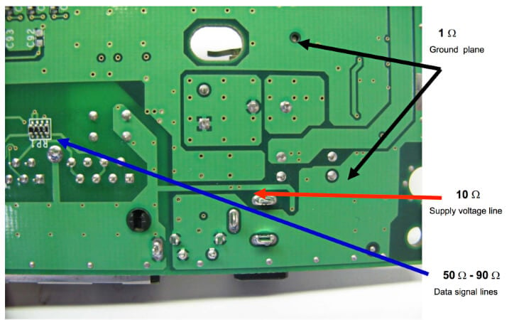
Figure 6. Different application types shown on a board.

 

Remember that these system impedance values are approximations, not exact representations for everything. But as you will see, for our purposes, the approximations work just fine and actually save us a lot of time. Most importantly, they save us from having to do those painful calculations!

 

Applying What We’ve Learned

Let’s walk through a quick example to apply what we’ve talked about. 

For this example, we released an EMI test in a chamber, and the test came back negative. Our board didn’t pass the test, and therefore we don’t have the right certification to release our product on the market. For a successful product launch we...

• Require 12dB of attenuation at 125 MHz
• Know that the issue came from the power cable 
• Know the power port has 10 Ω of impedance

First, we’ll try testing our math skills. You can see in the equation for filtering (ZF) that we can plug in these values, and the result is a filter impedance of 59.6 ohms. Then, if you are feeling up to it, you can double-check your work with the equation for attenuation (A). The result is 11.99 dB.

 

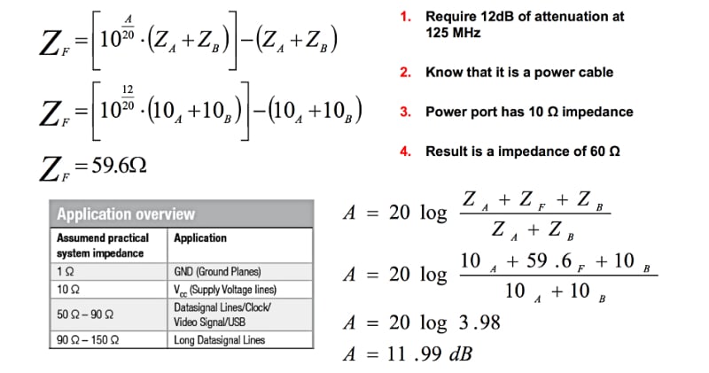
Figure 7. Calculations for the example problem.

 

Let's apply the same scenario, but this time using the nomogram. We quickly come up with the same conclusion without doing any complex mathematical equations.

Keep in mind that the frequency is part of the impedance equation. Therefore, you don't have to use the frequency when using a nomogram. You know you need 12 dB of attenuation (just like before), and you know it's a power cable (which means it has an impedance of approximately 10 ohms, according to our application overview table). 

 

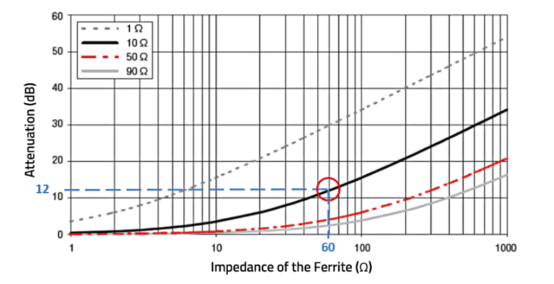
Figure 8. Nomogram showing the results from the example problem.

 

Simply follow the black solid line for supply voltage applications until it reaches 12 dB. There, you find your result of 60 ohms impedance — the requirement we already determined.

The answer came out the same for both the nomogram and the long mathematical calculations. Nomograms make the process a bit quicker and are provided in the Würth Elektronik catalogs for your convenience. Whichever method you choose to use, you now know how to easily calculate insertion losses in EMC!

In the next article in our series on EMC basics, we’ll cover the differences between common mode and differential mode noise and solutions for how to combat them. Stay tuned!

 

Würth Elektronik

Author: Dheeraj Jain, Technology Strategist; Jenna Cummins

EMC components: we-online.com/catalog/en/pbs/emc_components

Filter Designer: we-online.com/redexpert