Introduction to the Threshold Effect in FM Systems

We previously derived an expression for signal-to-noise ratio (SNR) in frequency modulation (FM) systems. Our findings in that 2-part article indicated that increasing the deviation ratio D enhances the output SNR, but this improvement comes at the cost of greater bandwidth consumption. This highlights a fundamental principle in FM system design: the trade-off between spectral efficiency and noise resilience.

This article explains that the commonly used FM SNR equation holds only when the input carrier-to-noise ratio (CNR) is sufficiently high. When the CNR falls below a critical threshold, the resulting SNR drops sharply and deviates from the value predicted by the standard equation. This threshold effect places an upper bound on how effectively bandwidth can be traded off against power in FM systems.

 

Key Assumption in FM SNR Derivation

The previous article analyzed the performance of the FM scheme in the presence of additive white Gaussian noise with a zero mean and a double-sided power spectral density of N₀/2 Watts/Hz. This resulted in the following FM SNR equation:

$$SNR_{out} = \frac{P_{s,out}}{P_{n,out}} = \frac{3 A_c^2 \times k_{f}^{2} \times P_{m}}{2 \times N_0 W^3}$$

Equation 1

where:

A_c denotes the carrier amplitude

P_m is the average power of the message signal

k_f is the frequency deviation constant

W is the message bandwidth in hertz.

An essential assumption is that the carrier amplitude remains much greater than the noise amplitude for the majority of the time. That is, the CNR is high. For reference, the CNR equation is given by:

$$\rho = \frac{A_c^2}{2 N_0 B_T}$$

Equation 2

 

where B_T denotes the FM signal bandwidth.

 

High CNR Assumption Leads to Additive Output Noise

Noise analysis is easier when circuit output consists of additive signal and noise components, as this allows for straightforward computation of the SNR. FM is inherently nonlinear, causing the signal and noise at the output to be so intermingled that they cannot be treated as additive components, even when the input noise is additive.

The assumption of a high CNR allows us to approximate the nonlinear FM process using an additive model. Although the assumption isn’t strictly valid in all cases, it’s frequently adopted in studies of nonlinear modulation systems. The remainder of this article explores the noise performance of FM systems under conditions where the high CNR assumption no longer holds.

 

What Is the Threshold Effect?

As discussed in the previous article, the SNR expression presented in Equation 1 can be rewritten in terms of the CNR as follows:

$$SNR_{out} = 3 \times D^2 \times \underbrace{\frac{P_{m}}{ \big ( Max(|m(t)|) \big )^2}}_{\text{Power of Normalized Message}} \times \frac{B_T}{W} \times \rho$$

Equation 3

 

For a given message signal and deviation ratio D, all terms on the right-hand side remain constant except for the CNR ⍴, which depends on the carrier amplitude and noise power. In this case, one might expect the output SNR to vary linearly with ⍴. However, this linear relationship breaks down in practice as ⍴ approaches a threshold value.

Figure 1 below shows the output SNR versus ⍴ for a typical FM system across multiple modulation index values. As the CNR decreases from high to low values, the output SNR initially decreases linearly but then drops sharply beyond a certain point. This critical CNR value is known as the threshold.

 

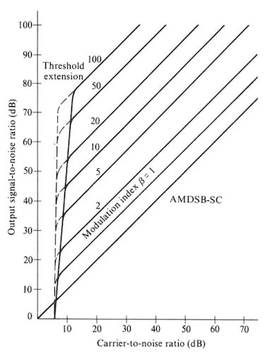
Figure 1. Output SNR versus the CNR for a typical FM system. Image used courtesy of Jerry D. Gibson.

 

When the system operates near the threshold value for a curve, even minor fluctuations in the received signal power can lead to significant changes in the system’s SNR. This means that near the threshold CNR, one moment the signal is successfully received, and the next it’s obscured by the noise.

As observed, the threshold depends on the modulation index β, or more generally on the deviation ratio D. Higher values of β result in a higher threshold. A typical threshold value is approximately 10 dB.

 

Qualitative Insights into the Threshold Effect

To understand the threshold effect, consider an FM wave in the presence of band-limited noise centered around the carrier frequency. It can be represented by the following equation:

$$s(t) + n_{filtered}(t) = A_c cos\big(2\pi f_c t + \phi(t)\big) + r_n(t) cos\big(2\pi f_c t + \phi_n(t)\big)$$

Equation 4

 

The first term on the right-hand side of the equation denotes the modulated carrier. The second term corresponds to the noise component expressed in polar coordinates.

Let’s take a look at the phasor diagram of the above equation when ϕ(t) = 0 and the noise is much smaller than the carrier, as illustrated below.

 

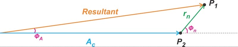
Figure 2. Phasor diagram representation of the noisy FM wave when CNR is high.

 

As the noise component varies randomly in amplitude and phase over time, the resultant vector’s tip (P₁) moves around the carrier vector’s tip (P₂). In the case of high CNR, the noise component is small, and point P1 spends most of its time near point P₂.

You should be able to visualize that even a dramatic phase swing in the noise vector, such as π radians, causes only a modest shift in the resultant vector’s phase because the carrier amplitude is significantly greater than that of the noise.

Now, we examine the phasor diagram corresponding to a low carrier-to-noise ratio. In this case, the carrier and noise amplitudes are comparable, and noise fluctuations can cause significant spikes in the demodulated FM output. This is illustrated in Figure 3 below.

 

Figure 3. Phasor diagram representation of the noisy FM wave when the CNR is low.

 

In the above diagram, the carrier vector is assumed to have zero phase, ϕ(t) = 0, throughout the interval from t₁ to t₂. At t = t₁, the phase of the noise vector ϕ_n(t) is close to -π radians, leading to the resultant vector’s phase being approximately -π radians. At t = t₂, the phase of the noise vector changes to ϕ_n(t) ≈ +π radians through the dashed locus, causing the resultant vector’s phase ϕ_A(t) to be approximately +π radians.

As observed, variations in the noise vector can cause point P₁ to occasionally sweep around the origin, resulting in a phase increase or decrease of 2π radians. Figure 4, generated using MATLAB, illustrates how the phase of the resultant vector, ϕ_A(t), evolves when random noise is added to an unmodulated carrier.

 

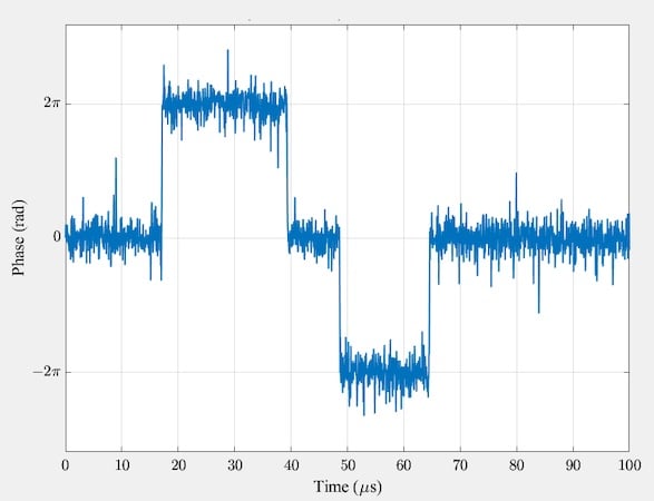
Figure 4. Phase variation of the noisy FM signal at CNR = 3 dB.

 

Under low CNR conditions, the phase of the resultant vector exhibits abrupt transitions of ±2π radians, corresponding to the threshold effect described earlier. Between these jumps, the phase fluctuates continuously due to the underlying band-limited noise. The resulting waveform includes small-scale fluctuations and occasional large discontinuities.

Since the demodulator produces the time derivative of the input phase, we expect the phase step changes of ±2π radians to generate sharp, impulse-like variations at the output. The derivative of the above waveform is shown in Figure 5.

 

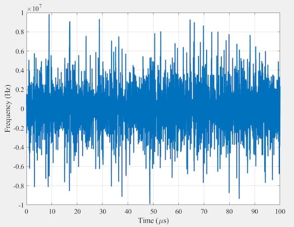
Figure 5. Instantaneous frequency extracted from the phase waveform in Figure 4.

 

The waveform contains many impulse-like variations of varying magnitudes. Most of these impulses arise from small-scale fluctuations in the resultant vector’s phase ϕ_A(t) rather than from abrupt ±2π transitions.

In its current form, the instantaneous frequency waveform is difficult to relate directly to the phase signal. By applying a lowpass filter to suppress high-frequency noise, we obtain a smoothed waveform that more clearly reflects the underlying phase behavior. This step is justified by the fact that practical FM demodulators incorporate a lowpass filter at the output to limit the noise bandwidth to that of the message signal. The lowpass filter used in my simulations has a bandwidth of 500 kHz, which appears to be higher than what is typically employed in practical FM demodulators.

The lower curve in Figure 6 shows the filtered instantaneous frequency. The upper curve reproduces the phase waveform to facilitate comparison between the two.

 

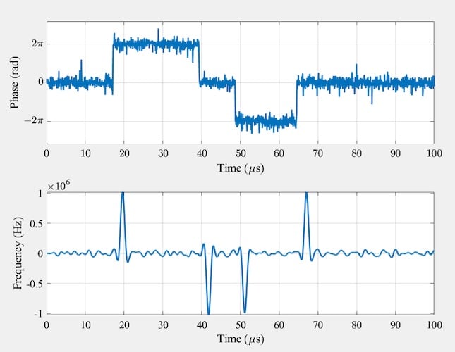
Figure 6. Resultant vector’s phase (top) and lowpass-filtered instantaneous frequency (bottom) at CNR = 3 dB.

 

We observe that abrupt phase deviations of ±2π radians at the input produce sharp, impulse-like variations at the output. From linear systems theory, it follows that the areas of these impulses are nearly equal to ±2π radians.

 

Why Are These Impulses Problematic?

These spikes would manifest on an FM radio as a crackling or clicking noise. When the CNR is gradually reduced, the receiver initially produces occasional clicks. As the CNR drops further, the average number of clicks per unit time increases.

When this number becomes appreciably large, the threshold effect is said to occur. At this point, the clicks merge into a crackling sound and obscure the signal. Figure 7 shows the results for a lower CNR value of 0 dB, confirming an increase in the average number of impulses.

 

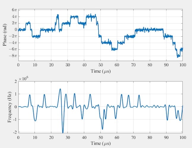
Figure 7. Resultant vector’s phase (top) and lowpass-filtered instantaneous frequency (bottom) at CNR = 0 dB.

 

The occurrence of spikes in the output suggests that the output noise spectrum is no longer parabolic. The spikes generate notable low-frequency content. In the presence of the threshold effect, the output SNR degrades abruptly and no longer follows the prediction of the standard formula (Equation 1).

 

Wrapping Up

In this article, we examined the threshold effect in FM systems, showing how a sudden and dramatic degradation in signal quality occurs once the CNR drops below a critical level. Our analysis showed that below this threshold, the noise effectively captures the desired FM signal, producing impulsive spikes at the demodulator output that drive the SNR significantly lower than predicted by the standard SNR equation. In the next article, we’ll explore this phenomenon further and show that it imposes a fundamental limit on the trade-off between bandwidth and power in FM systems.

 

Feature image background used courtesy of Adobe Stock.