Performing Worst-Case Circuit Analysis with LTspice

This article will discuss how to use LTspice, a powerful SPICE simulation tool from Analog Devices, specifically for worst-case analysis (WCA). This type of analysis helps ensure that a newly-designed circuit is compliant with all the requirements under every circumstance—i.e., considering temperature variations, component tolerances, aging, and derating, among other factors.

Using the stepped variation of parameters, this tool can also be useful to see which components have larger effects on the measurements. As an example, we'll analyze a resistive circuit for a temperature sensor reading to show the powerful results of this tool and technique. 

 

What is Worst-Case Analysis?

While the title "worst-case analysis" sounds self-explanatory enough, some aspects of this method merit further discussion. Worst-case analysis is a numerical method that assesses whether a new circuit or system will be compliant with requirements throughout the duration of the project.

In some mission-critical sectors, such as the space industry, this method can help ensure that an electronic system designed today will be fully functional in 2050 or later. 

 

Temperature Sensor Reading for NTC Thermistors

Negative temperature coefficient (NTC) thermistors are resistors with values that are inversely proportional to the temperature. They are widely used because of their low price, simplicity, and easiness to mount. The Steinhart-Hart equation approximates the temperature based on the resistance value:

 

\[\frac {1}{T}=A+Bln(R)+C(ln(R))^3\]

 

Constants A, B, and C depend on the type of thermistor and the manufacturer supplying the thermistor. 

The following equation is less accurate but easier to use. 

 

\[\frac{1}{T}=\frac{1}{T_0}+\frac{1}{\beta}\ln\left(\frac{R}{R_0}\right)\]

 

R₀ is the resistance at the reference temperature T₀. The parameter \(\beta\), which is reported in kelvin (K), is available from the manufacturer and is usually included in the datasheet. For more details, you can review this chapter on NTC thermistors. 

We can obtain the temperature by measuring the NTC resistance and knowing the \(\beta\) parameter.  For our purpose, we are going to use the NTC Murata NCU15XH103F6SRC, which has a resistance of 10 kΩ at 25ºC and \(\beta\) parameter 3380 K.

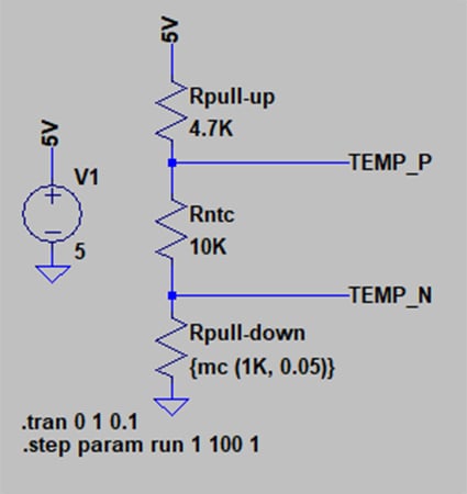
It is common to use the following circuit to get the resistance value of a thermistor. 

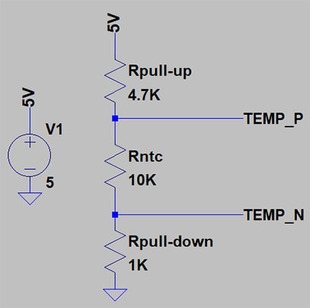
Setup to measure temperature with a thermistor.

 

This can be achieved by measuring the voltage drop across the thermistor.

The voltage at node TEMP_P is

 

\[V_{NTC}=V_{cc}\frac{R_{ntc}+R_{pull-down}}{R_{ntc}+R_{pull-down}+R_{pull-up}}\]

 

Knowing this voltage, we can calculate the NTC resistance. Then, we can calculate the measured temperature. 

 

What Other Parameters Affect Measurements in a Circuit?

The presented circuit has only three passive components, but there are quite a few parameters that can affect the measurement, like passive component tolerance and power supply bouncing. These factors must be taken into account as well.

 

Passive Component Tolerance

Real components are not perfect; they have a tolerance, stated by their manufacturer. Frequent values are 1% or 5%.

5% tolerance means that a 1 kΩ resistor can have any resistance value between 950 Ω and 1050 Ω. When a circuit has many resistors, the cumulative effect of the tolerance can produce a result far from what you expected.

 

Power Supply Bouncing

Power supplies are made to be stable, but like passives, they have their faults. If we are doing a measurement that depends directly on the voltage supply, we need to know the voltage variations. For our purposes, we will consider a 5 V supply that varies between 4.9 V and 5.1 V.

 

Modifying a Parameter in LTspice

One way to study different situations in LTspice is to change parameters manually and then repeat the simulation each time. This process can be time-consuming and error-prone. LTspice has various methods to change settings and simplify multiple simulations.

 

STEP and Monte Carlo Commands in LTspice

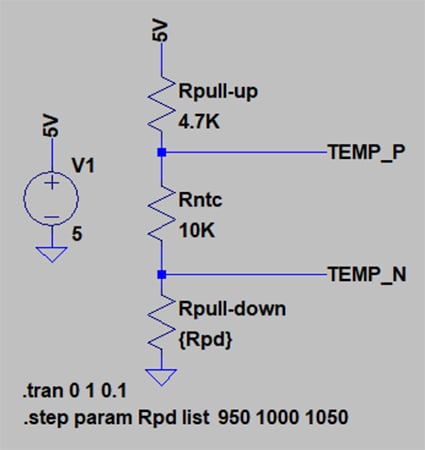
The STEP command automatically performs the variation of the desired parameters and simulates each one. This is accomplished by placing the component value between brackets—for example {Rpd}—and adding a SPICE directive:

• Using .step param Rpd list 950 1000 1050, the simulation will run with each of the three listed values. We are going to use this directive.
• Using .step param Rpd 950 1050 50, the simulation will run from the lowest level to the highest in steps of 50.

 

STEP parameter greatly reduces the time for analysis.

 

There is a second option to make parameters change.

The MC command stands for Monte Carlo analysis. It can achieve more than the STEP command since the latter requires the designer to know all the discrete values of each component while the Monte Carlo analysis performs a statistical analysis. In each iteration, Monte Carlo analysis returns a random number within the tolerance interval.

To set up a Monte Carlo analysis for the \(R_{pull-down}\) resistance, we need to define its component value as follows: {mc (1K, 0.05)}. Furthermore, we need a SPICE directive: .step param run 1 100 1. This means that the simulation will run one hundred times, starting with one and with steps of one.

 

Any component of the circuit can be included in a Monte Carlo analysis.

 

Parameter variations are not restricted to just one component. We can define all the parameters we want. We can also define constants, such as tolerances, so all the components are modified at the same time instead of typing each one by one. This is done with the directive .param. We will do it for tolR (0.05) and tolV (0.02). 

 

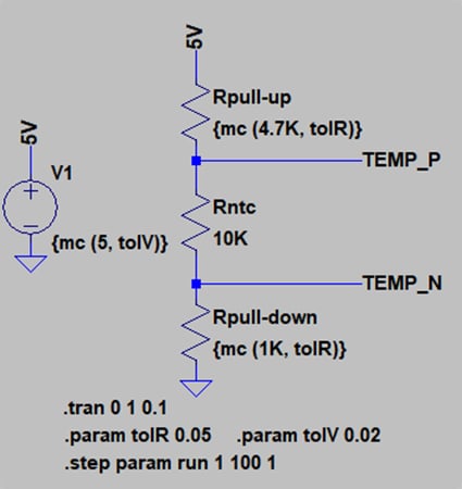
Constants allow the execution of complex simulations and reduce errors.

 

How to Plot the Results in LTspice

Once all the simulations are completed, we can plot the results. To directly view the NTC voltage, we do the following:

1. Right-click at TEMP_N and select “Mark reference.” We will see a black probe over the net.
2. Left-click at TEMP_P. We will see the signal: V(TEMP_P, TEMP_N) and a group of colored lines; each of them corresponds to one simulation.

 

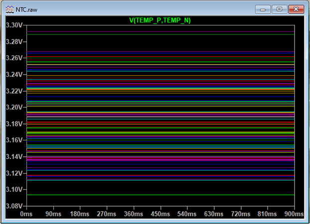
As the number of iterations increases, the entire tolerance interval is covered.

 

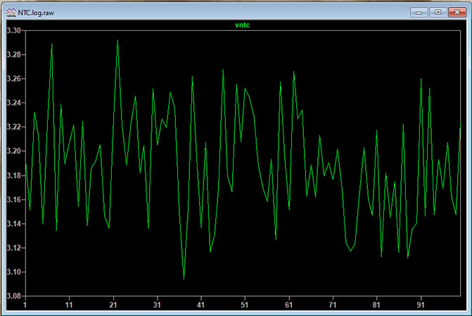
We can improve the analysis by adding some graphs. LTspice can draw graphs with user-defined independent variables. To represent the NTC voltage against the execution number, we need to follow these steps:

1. Place the directive: .measure Vntc AVG V(TEMP_P, TEMP_N)
2. Run the simulation again.
3. Menu View → Spice Error Log → Right-Click anywhere → Plot .step’ed .meas data

 

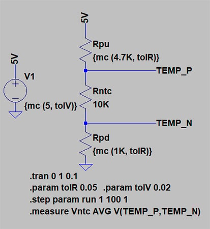
Measure command can measure average, RMS, maximum or minimum, and other factors. 

 

 

Conclusion

LTspice is a powerful tool. While its graphical interface can be discouraging, its capacity for simulations is well worth the effort to use the tool. Worst-case analysis is one of the necessary steps to perform when designing a new circuit. LTspice gives designers the functions and tools to perform precise and complex analyses.