 Facebook
 Google
 GitHub
 Linkedin
What an Electronics Engineer Needs to Know About Noise
In this article, we’ll try to develop insight into some of the most important characteristics of the noise sources that we commonly have to deal with in electronics engineering.
Noise is an unwanted disturbance that degrades the accuracy of our desired signal. To analyze the effect of noise on a system, we need to have a basic understanding of its behavior.
In this article, we’ll try to develop insight into some of the most important characteristics of the noise sources that we commonly have to deal with in electronics engineering.
Randomness
Noise is a random signal. This means that its instantaneous amplitude cannot be predicted based on its previous values. Figure 1 shows an example.
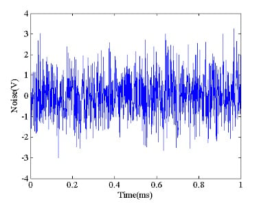
Figure 1
If the instantaneous amplitude of noise is not known, how can we determine its effect on a system output? Although the instantaneous amplitude is not predictable, there are other properties of the noise waveform that can be predicted. This is at least true for the noise sources that we commonly have to deal with in circuit design and analysis.
Let’s see what properties are predictable and how analyzing them can help us.
Histogram of Noise Amplitude
The first step in characterizing a noise source can be estimating how often a given value is likely to occur. To this end, we take a large number of samples from the noise waveform and create an amplitude histogram.
For example, assume that we have 100,000 samples from the noise waveform. Depending on the value of these samples, we can consider a possible range for the noise amplitude. Then, we divide the entire range of the possible values into a number of consecutive non-overlapping amplitude intervals called bins. The bins (intervals) of a histogram are usually of equal size. The height of a bin is determined by the number of occurrences of the noise amplitude values that are within the bin interval.
Figure 2 shows the histogram of 100,000 samples of a random variable. In this example, the histogram has 100 bins and the maximum and minimum sample values are 4.34 and -4.43, respectively.
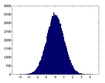
Figure 2
The above histogram shows how often the noise amplitude takes on a value within a given interval. For example, the histogram shows that values around zero are much more likely to occur.
Estimating the Amplitude Distribution
The information in the above histogram indicates the likelihood of having a particular amplitude value; however, it is based on a specific experiment where 100,000 samples are taken. We usually need a likelihood curve that is independent of the number of samples. Hence, we have to somehow normalize the information of Figure 2.
Obviously, all of the bin heights should be divided by the same value so that the obtained curve can still show the relative likelihood of the different amplitude intervals correctly. But what is the appropriate normalization factor? We can divide the bin heights by the total number of samples (100,000) to give the relative number of occurrences for a bin interval rather than its absolute value. However, another modification is still required before the curve represents a probability.
As mentioned earlier, the height of an interval indicates the total number of noise amplitude values that are within the continuous range of that interval. All of these values, within a given bin interval, are denoted using a single number that represents the interval likelihood. While the values of the histogram in Figure 2 denote the interval likelihood, in probability theory, we use a density connotation to specify the likelihood of a continuous variable. Thus, in order to have a curve that shows the probability density correctly, we should divide the bin heights by the bin width. This normalized curve is a rough estimate of the variable probability density function (PDF) which is a very important feature of the underlying random process.
We can arrive at this same result with a slightly different approach: According to our measurements, the noise amplitude is between -4.43 and 4.34. In reality, the noise amplitude can take a value outside this range; however, we are using our measured data to have an estimate of the amplitude distribution. For the rough model that we are developing, the event of having a value between -4.43 and 4.34 is absolutely certain to occur (its probability is 1).
This probability can be found by calculating the total area under the normalized curve (which is the estimated PDF). For the normalized curve to have a total area of one, we should normalize the bin heights by a factor equal to the total histogram area. The histogram area is equal to the bin width multiplied by the total number of samples. Hence, the normalization factor is equal to the bin width multiplied by the total number of samples. Applying this normalization factor gives us the estimated PDF shown in Figure 3.
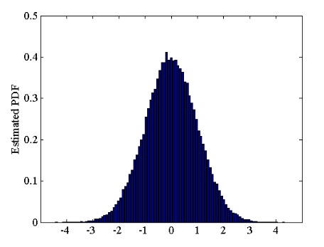
Figure 3
The Stationarity Assumption
The above discussion is based on a fundamental assumption. It assumes that a long observation of the random process can be used to estimate its distribution function. In other words, the distribution function from which our random signal originates doesn’t change over time. Actually, this is not the case in general but it is valid for the noise sources of interest to us. A random process is called stationary if its statistical properties do not change over time.
Calculating the Mean Value
The PDF of a random variable allows us to have an estimate of its sample mean. Let’s consider a simple example. Assume that a hypothetical random signal, X, has three possible values: 1, -2, and 3 with a probability of 0.3, 0.6, and 0.1 respectively. How can we find the mean value of this signal? One way is to estimate the mean value by taking a large number of samples from the signal. In this case, we can calculate the sample mean by calculating the arithmetic average of the data observations:
\[\bar{x}= \frac {1}{N} \sum_{i=1}^{N}x_i\]
where N denotes the total number of samples and xi denotes the i-th sample. Note that what we get is still an estimate of the random variable mean value because the signal is random and we cannot predict the future values. A better approach to estimating the mean value is based on using the probability of the different outcomes.
Based on the probability values given for this example, we can conclude that if we observe this random signal for a long time, it’ll have a value of 1 for about 30% of our observation duration. The signal will have values -2 and 3 for about 60% and 10% of our observation duration, respectively. Hence, we can use the probability of the different outcomes as a weight for that outcome. We obtain:
\[E(X)=1 \times 0.3 + (-2) \times 0.6 + 3 \times 0.1 = -0.6\]
where E(X) denotes the expectation of the random variable X. The expectation of a random variable can be thought of as an estimate of the mean value of the samples of a random variable. The expectation of the discrete random variable X is given by:
\[E(X)= \sum_{all \: \: x} xp(x)\]
where X denotes the random variable and x denotes the values that X can take on. p(x) represents the probability of X taking on the value x. For a continuous random variable, we have the following equation:
\[E(X)= \int_{- \infty}^{+ \infty}xp(x)dx\]
As you can see, the PDF allows us to predict the mean value of a noise waveform. The expectation of a random variable is sometimes represented by μ. We can plug in the exact values from Figure 3 to find the expectation value of this example; however, visual inspection reveals a symmetry around zero and we can predict that the mean value of this random variable is zero.
The Variance of a Random Variable
Similarly, we can use the PDF of a random variable to estimate its variance. If we had N samples from the random variable, we could use the following equation to find the sample variance:
\[s^2 = \frac{1}{N-1} \sum_{i=1}^N(x_i-\bar{x})^2\]
Note that the denominator is chosen to be N-1 rather than the more obvious choice of N. Please refer to Section 7.2.1 of Probability and Statistics for Engineers and Scientists by Anthony Hayter for an explanation of the use of N-1 rather than N.
Using the probability of a given outcome as a weight for the distance between that outcome and the mean value, we obtain:
\[E\left ( (x -\mu )^2 \right )=\sum_{all \: \: x} \left ( x - \mu \right )^2p(x)\]
For a continuous random variable, we have the following equation:
\[E\left ( (x -\mu )^2 \right )=\int_{- \infty}^{+ \infty} \left ( x - \mu \right )^2p(x)dx\]
Therefore, the PDF allows us to predict both the mean value and the variance of a noise waveform.
Variance and Average Power
For μ =0, the variance of a continuous random variable simplifies to:
\[E\left ( x^2 \right )=\int_{- \infty}^{+ \infty} x ^2p(x)dx\]
This is the expectation of the squared value of the noise samples. This value is conceptually similar to the average power of a deterministic voltage signal s(t) defined by
\[P_{avg} = \lim_{T \rightarrow \infty} \frac {1}{T} \int_{-\frac{T}{2}}^{+ \frac{T}{2}}s^2(t)dt\]
where the average power is expressed in V2 rather than W. The idea is that if we know Pavg, we can easily calculate the actual power delivered to a given load RL by dividing Pavg by RL. For a random variable, we don’t know the instantaneous sample values. However, we can use the expectation concept to predict the average value of x2. Therefore, for μ = 0, the variance of a noise waveform is an estimate of the noise average power.
As you can see, the PDF allows us to extract some precious information such as the mean value and average power of the noise component.
Although we are now able to estimate the average power of noise, there still remains one major question: How is the noise power distributed in the frequency domain? The next article in this series will look at this issue.
Conclusion
Noise is an unwanted disturbance that degrades the accuracy of our desired signal. To analyze the effect of noise on a system, we need to have a basic understanding of its behavior. The instantaneous amplitude of noise cannot be predicted; however, we can still develop a statistical model for the noise sources of interest to us. For example, we can estimate the mean value and average power of noise. This information along with the noise power spectral density (PSD) are usually adequate to analyze the effect of noise on the circuit performance.
To see a complete list of my articles, please visit this page.


Good article, well written and easy to understand. I remember I learned about all this at university, but I find this article more explanatory. Useful for electronic engineering students.