 Facebook
 Google
 GitHub
 Linkedin
RF Design Basics—Introduction to Transmission Lines
Learn about voltage waves and how they relate to an important basic concept of radio frequency (RF) circuit design: transmission lines.
One important factor in circuit design is the physical dimensions of the circuit elements and interconnects with respect to the wavelength of the signal being processed. When the signal frequency is low enough so that the physical dimensions of the interconnect are less than about one-tenth the signal wavelength, we can assume that different points along the wire are at the same potential and have the same current.
From a practical point of view, this is a satisfactory assumption that significantly simplifies the low-frequency circuit design. However, as we go to higher frequencies, we might need to describe the signal as a wave traveling along the wire. In this case, the signal magnitude is a function of both time and position.
The Signal of a Voltage Wave Traveling Along a Wire
As an example, consider applying a sinusoidal input Vscos(⍵t) with a source impedance of Rs to a load impedance RL through a pair of long wires (Figure 1(a)).
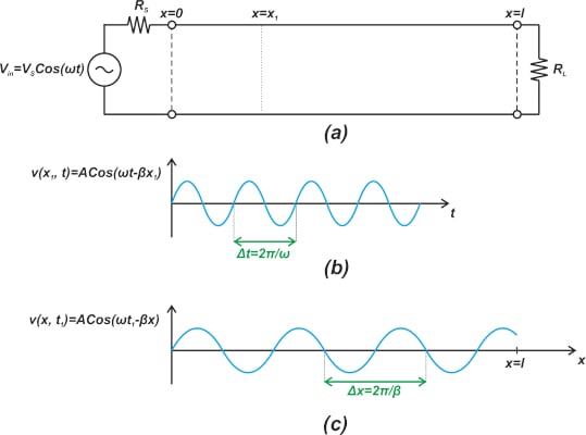
Figure 1. An example using a pair of long wires (a), a waveform of a sinusoidal function of time (b), and a waveform showing the voltage along the wire (c).
Suppose that the wire, which is in the x-axis direction, has a length much greater than the signal wavelength. Also, assume that the interconnect has a uniform structure and different parameters, such as the conductor dimensions, the spacing between the conductors, etc., are the same along the wire.
The steady-state voltage and current signals that appear along the wire depend on the value of a number of parameters; however, in order to paint a qualitative picture of this circuit’s behavior, we’ll assume that the voltage wave can be described by Equation 1:
\[v(x,t)=Acos(\omega t- \beta x)\]
Equation 1.
Where A and β are some constants that depend on the circuit parameters. As shown, the voltage signal is a function of both time (t) and position (x). At a fixed position x = x1, the βx term is a constant phase term, and the above waveform is simply a sinusoidal function of time (Figure 1(b)). The period T of this sinusoidal function is:
\[\omega \Delta t=2 \pi \Rightarrow T = \Delta t= \frac{2 \pi}{\omega}\]
To examine the waveform dependency concerning position, we can look at the waveform at a particular instant in time t = t1. In this case, the term ⍵t turns into a constant phase term, and we observe that the voltage signal is a sinusoidal function of position x. The example waveform in Figure 1(c) shows how the voltage along the wire varies sinusoidally along the interconnect at a given point in time. This waveform can be considered a periodic function of x over the wire length. The period is given by:
\[\beta \Delta x=2 \pi \Rightarrow \Delta x= \frac{2 \pi}{\beta}\]
The above equation specifies the distance between two consecutive equal values of the signal along the wire at a given moment of time. This is actually the definition of the wavelength that is commonly denoted by Equation 2:
\[\lambda= \frac{2 \pi}{\beta}\]
Equation 2.
Direction and Speed of Propagation
Just like water waves that travel in a particular direction, electrical waves also propagate in a specific direction. As an example, consider the wave function in Equation 1. At a given time (t2), the function value at position (x2) is:
\[v(x_2,t_2)=Acos(\omega t_2- \beta x_2)\]
With that in mind, assume that this value corresponds to point A in Figure 2(a).
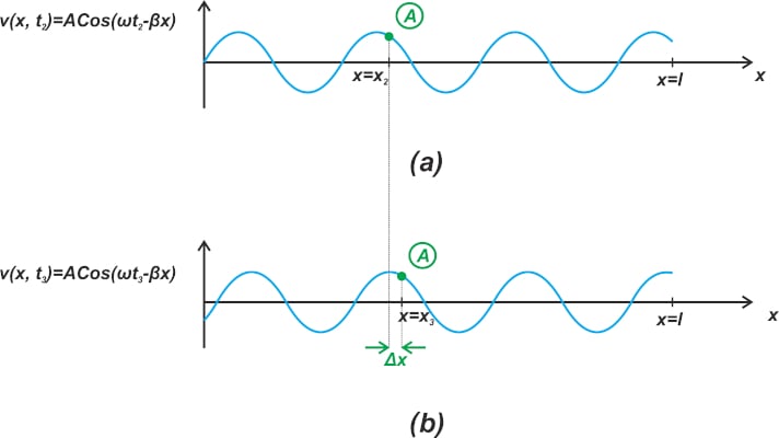
Figure 2. Example waveforms where (a) shows the position (x2) is A, and (b) shows the position (x3) is A. which shifts to the right.
In what direction point A is going to move as time passes? If the next position of point A is x3 at time, t3, (Figure 2(b)), we should have:
\[v(x_3,t_3)=v(x_2,t_2) \Rightarrow cos(\omega t_3- \beta x_3)=cos(\omega t_2- \beta x_2)\]
Which simplifies into Equation 3:
\[\omega t_2- \beta x_2 = \omega t_3- \beta x_3 \Rightarrow \frac{x_3-x_2}{t_3-t_2}=\frac{\omega}{\beta}\]
Equation 3.
Assuming that β is a positive value and noting that t3 > t2, x3 should be larger than x2. In other words, point A travels in the positive x direction. However, you might wonder, what about the following wave function in Equation 4?
\[v(x,t)=Acos(\omega t+ \beta x)\]
Equation 4.
The next position of a given point on this wave corresponds to the x value that keeps ⍵t + βx constant. Since the term ⍵t increases with time, x should decrease. Therefore, this wave travels in the negative x direction. Equation 3 actually gives the speed of propagation (also known as the phase velocity (vp) of the wave):
\[v_p = \frac{\omega}{\beta}\]
RF Wave Reflection
Fortunately, various types of waves, including mechanical, electrical, acoustical, and optical waves, behave fundamentally alike. This helps us to use our intuition from more tangible types, such as a water wave, to better understand the behavior of the other types. One similarity of waves of all kinds is that they reflect when certain properties of the medium they are traveling through change.
For example, when a water wave traveling toward the shore collides with a rock, it reflects off it and propagates back into the ocean. Similarly, a voltage wave reflects when the impedance of the wave medium changes.
In the example depicted in Figure 1(a), the wave traveling in the positive x direction reflects when the load impedance RL is not matched to a special property of the interconnect called characteristic impedance (often denoted by Z0). Upon reflection, a wave in the negative x direction is created that travels from the load toward the voltage source. Therefore, in general, we can expect the incident and reflected waves to travel simultaneously along the wire. The ratio of the reflected voltage to the incident voltage is defined as the reflection coefficient and is denoted by $$\Gamma$$.
Impedance Matching: RF Engineer’s Obsession
Since some of the incident power is reflected back to the source, the load cannot receive the maximum power that the source provides. Therefore, the reflection coefficient is an important parameter that determines how much of the available power is actually going to reach the load. To achieve maximum power transfer, the load impedance should match the characteristic impedance of the line.
Another issue with load mismatch is that the superposition of the incident and reflected waves can create large peak voltages along the wire that can damage our circuit components or interconnects. The above discussion shows that when dealing with high-frequency signals, we need interconnects with precisely controlled parameters to predict the wave behavior as it travels along the interconnect. For example, the dimensions of the conductors, the distance between them, and the type of dielectric that separates the conductors should be precisely controlled. These specialized interconnects are called transmission lines to distinguish them from ordinary interconnects.
RF Wave Dimensions
As a rule of thumb, if the physical length of a wire is about $$\frac{\lambda}{15}$$, the electrical signal should be considered as a wave traveling through the wire.
Figure 3 helps you visualize how restricting the wire length to $$\frac{\lambda}{15}$$ reduces the signal variations with the position.
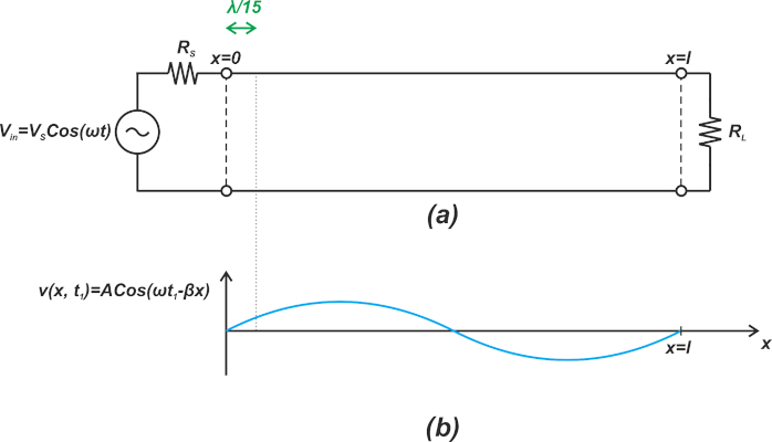
Figure 3. An example showing how, by restricting wire size (a), the signal varies with the position (b).
Some references suggest a physical size of $$\frac{\lambda}{10}$$ as the threshold at which the signal variation with position is expected to be significant.
Now that we have a qualitative understanding of electrical waves and transmission lines let’s take a look at the equivalent circuit of a transmission line and see how we can eliminate reflections.
Transmission Line Equivalent Circuit
When the wire dimensions are comparable with the wavelength, we are dealing with electrical waves traveling along the wire. In this case, Kirchhoff’s circuit laws (law of voltage and law of currents) cannot be directly applied. However, we can still find an equivalent circuit for two-conductor interconnects at high frequencies. To this end, the line is divided into elements of infinitesimal length, and each element is modeled as a network of an inductor, a capacitor, and two resistors. This is illustrated in Figure 4.
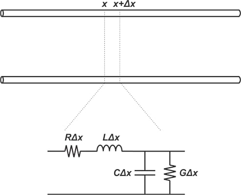
Figure 4. An example showing a transmission line's elements: an inductor, capacitor, and two resistors.
Here, R and G represent, respectively, the resistance per unit length of the wire and the conductance per unit length of the dielectric that separates the conductors. L and C represent the inductance and capacitance per unit length of the transmission line.
At radio frequencies, the series reactance is usually much greater than the series resistance, and the shunt reactance is usually much less than the shunt resistance, so we can assume that both resistances can be neglected. Neglecting R and G components, a lossless transmission line can be modeled by the infinite ladder network shown in Figure 5.
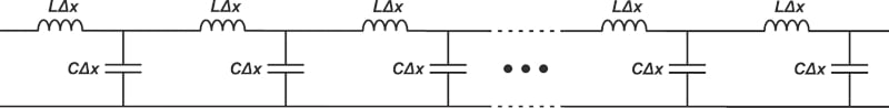
Figure 5. A model of an infinite ladder network.
Eliminating Reflections Via Impedance Matching
With a transmission line of infinite length, the incident wave would travel in the forward direction forever, and there would be no reflection! Let’s see if we can emulate this theoretical situation by appropriately choosing the parameters of a real finite-length transmission line. For an infinitely long transmission line, there is an infinite number of segments in the equivalent circuit, which we saw in Figure 5.
If we add another infinitesimal section to this infinite ladder network, the input impedance should remain unchanged. In other words, if the diagram in Figure 6 corresponds to an infinitely long transmission line, the input impedance “seen” from nodes A and B are the same.
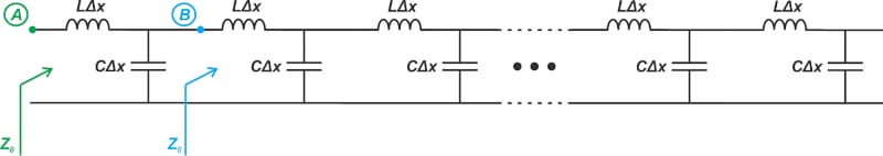
Figure 6. An example of an infinitely long transmission line.
Therefore, we can simplify the above diagram, as shown in Figure 7.
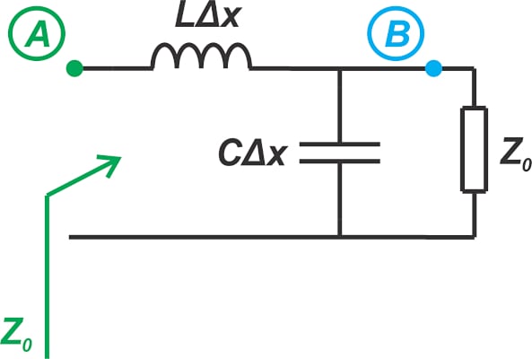
Figure 7. A simplification of Figure 6's infinitely long transmission line example.
From this diagram, the input impedance is:
\[Z_0 = L \Delta x s+\big( \frac{1}{C \Delta x s} \parallel Z_0 \big)\]
Using a little algebra, we obtain:
\[CZ_{0}^2-L-LC \Delta xZ_{0}s=0\]
Since Δx $$\rightarrow$$ = 0, we can ignore the third term, leading to:
\[Z_0 = \sqrt{\frac{L}{C}}\]
The above equation gives the input impedance for an ideal, lossless, infinite transmission line. Since this is an important property of a transmission line, it is given a special name: the characteristic impedance of the transmission line. How can we use this information to eliminate reflections in a finite-length transmission line? As we discussed above, the circuits in Figures 6 and 7 are equivalent from the source's perspective. This suggests that if we terminate a transmission line to a load resistor equal to the characteristic impedance of the line, the transmission line will appear as an infinitely long line from the perspective of the source, and no reflection will occur.
A Network of Reactive Components That Dissipates Energy!
It’s interesting to note that while the whole network consists of reactive elements, the input impedance is a positive, real value. Purely reactive elements are incapable of dissipating power; however, the above analysis shows that the whole network can be modeled by a resistor, and thus, it is dissipating energy!
The answer lies in the fact that the network is assumed to be of infinite length. Such a structure is an interesting abstraction but physically impossible. In an infinite transmission line, the energy keeps traveling down the line forever. It is not consumed by any of the inductors or capacitors. The line acts like a black hole for energy.
When we set RL = Z0, the load resistor dissipates energy eternally in the same way a transmission line of infinite length can eternally absorb energy. As a result, the reflections are omitted.
To see a complete list of my articles, please visit this page.


Dr. Arar, nicely explained tutorial on RF transmission lines!