 Facebook
 Google
 GitHub
 Linkedin
Embedded Firmware Tips: Converting Digital Signal Waveforms into Code with Scilab
This article describes a simple procedure that helps you to introduce a wide variety of signals and mathematical functions into your microcontroller projects.
A 25 or 50 MHz microcontroller equipped with an analog-to-digital converter and a digital-to-analog converter is by no means incapable of performing serious signal-processing and signal-generation tasks. And actually, MCUs should be recruited for DSP applications whenever possible, because they’re less expensive and easier to use.
Learn how to use Scilab to facilitate communication between your PC and your MCU code and also modify data.
Digital Signal Processing with Microcontrollers
One possible obstacle, though, is the difficulty of incorporating the required signals and mathematical waveforms into the firmware. I imagine that high-end digital-signal-processor development suites have sophisticated tools that help engineers to handle this aspect of DSP design, or perhaps employees working in larger engineering firms have an abundance of existing code or data files from which they can copy and paste.
In contrast, microcontrollers are often accompanied by development tools that are more basic and professional environments that are...well, less professional. When we’re designing with MCUs, we often have to work more independently and make do with limited resources.
This article will discuss a technique that can make your MCU-based signal-processing workflow much more smooth and satisfying. More specifically, I’ll show you a way to conveniently move waveform data from a PC to a typical C-language code file.
Storing Signals and Waveforms
First, let’s review the basic format that we can use for numerical sequences. Signals and waveforms will be stored as elements in an array, and we can initialize an array with the required numerical values as follows:
unsigned char Signal[100] = {Value1, Value2, Value3, …, Value99, Value100};
For example, a 20-element sine-wave cycle would look like this:
float Signal[20] = {0.000, 0.309, 0.588, 0.809, 0.951, 1.000, 0.951, 0.809, 0.588, 0.309, 0.000, -0.309, -0.588, -0.809, -0.951, -1.000, -0.951, -0.809, -0.588, -0.309};
This is what the signal’s numerical values look like in visual form:

Our objective here is to easily change the numbers inside the curly brackets. The numbers themselves will come from a PC and could be sensor data, mathematically generated data, measured data that has been processed by a filter, and things of that nature. We want to bridge the gap between the microcontroller code, which is really just a text file, and the PC, which has a convenient user interface and abundant processing resources.
Before we move on, I want to point out a related tip: It is often a good idea to store these types of arrays in code memory. This allows you to store relatively large amounts of DSP data without consuming all of your RAM resources. Please refer to [[this previous tips and tricks article]] for more information.
Generating Numerical Text with Scilab
In this article, I will use Scilab as the mediator between the PC and the MCU code. Other software (MATLAB, Excel, etc.) could be used, but Scilab is a good choice because it’s free, powerful, and fairly intuitive. The first step is to get your data into a Scilab array. You can import data from a file or generate it using Scilab’s mathematical functions. (This plot digitizer website might be helpful; I’ve never used it, so I’m not sure.)
It is also possible to manually enter data, either via typing or copy and paste, into a spreadsheet representation of the array; for example:

If you want to modify the data—apply a FIR filter to remove noise, increase the amplitude, change the sampling rate, etc.—now is the time. When the data is ready to become part of the microcontroller firmware, the final step is to generate a text file from which you can easily copy the values and then paste them into the code file.
To do this, we will use Scilab’s csvWrite() function.
Here’s an example:
filename = fullfile(TMPDIR, "data.txt");

csvWrite(SineWaveCycle, filename, ", ", ".", "%.3f");
The fullfile() command creates a “data.txt” file in a directory that you can find by double-clicking on the “filename” variable in the Variable Browser:

The first argument in the csvWrite function is the name of the array that holds the data. Next is the filename. The third argument specifies the characters that will separate the data values; the default is a comma, but for aesthetic purposes I changed it to a comma followed by a space. The fourth argument in my csvWrite command tells Scilab to use a period (rather than a comma) for the decimal mark, and the fifth argument specifies a precision of three decimal places.
Here is the result:
0.000, 0.309, 0.588, 0.809, 0.951, 1.000, 0.951, 0.809, 0.588, 0.309, 0.000, -0.309, -0.588, -0.809, -0.951, -1.000, -0.951, -0.809, -0.588, -0.309
Now all you need to do is copy all this and paste it between the array-initialization curly brackets in the code file. Whenever you need to modify the data, just close the text file, use the same cvsWrite command, open the file, and copy and paste.
Conclusion
I hope that you enjoyed this simple firmware-development technique and that it proves to be useful for you. Feel free to leave a comment if you have any related tips that you would like to share.
Related Content


unsigned char Signal[20] = {0.000, 0.309, 0.588, 0.809, 0.951, 1.000, 0.951, 0.809, 0.588, 0.309, 0.000, -0.309, -0.588, -0.809, -0.951, -1.000, -0.951, -0.809, -0.588, -0.309};
Did you actually mean float Signal[...].... instead?