Facebook
 Google
 GitHub
 Linkedin
Modeling Hysteresis in SPICE
Modeling hysteresis in SPICE can be difficult when you're dealing with a multivalued transfer function. In this article, we'll teach you a way to "cheat" to get around this issue.
This article provides a technique for the construction of standard SPICE models that are able to model the essential characteristics of systems with continuous hysteresis.
The example model in this article shows the addition of high-frequency sine wave bias to an audio signal to reduce the distortion of signals on an analog tape recorder. The technique allows for a sufficiently accurate approximation that illustrates hysteretic-generated distortion and how it is reduced by the addition of high-frequency bias.
A Hysteresis Model
The essential problem of modeling hysteresis is that it is a static or DC effect that has memory. That is, the next value depends not only on the present value, but also on the last value. However, this last value dependence does not depend on time. This results in a multivalued transfer function.
Unfortunately, standard SPICE does not directly support this type of modeling. All dependence on the last value in SPICE is usually the result of a linear integration, which inherently results in frequency-dependent transfer function and no account of distortion mechanisms.
A way around this problem is to simply recognize that one can cheat. Analog models only have to do what they need to do, approximately, over a finite range of frequencies. Analysis shows that a small capacitor in conjunction with nonlinear diode resistances can be used to continuously store the last value of a signal before it changes slope direction to provide an effective hysteresis, but without unduly being dependent on frequency.
This is in contrast to some SPICE “hysteresis” models that are only two output state models that do not allow for a continuous transfer function.
The Linear Model
The following schematic forms the basis of a continuous hysteresis model that may be used for modeling; for example, magnetic cores.
Note that here the output voltage is multivalued but, essentially, linear outwith the deadband. A deadband is generated when the signal changes direction. It can be adjusted with the diode parameter, N.
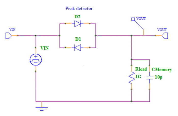
Figure 1. Schematic of a continuous hysteresis model
The output voltage of this block, essentially, linearly follows the input, but with an offset voltage. When the input turns around, the capacitor holds the voltage such that there is a deadband starting from the peak voltage reached.
The key principle of operation is that there is nonlinear impedance that has a sharp ratio of resistances for forward and reverse bias conditions. The standard diode equation is the simplest, but not a necessary equation for the technique. It is used here to illustrate the method.
Alternative equations may be used to fine tune the response characteristics. The input voltage may also be further processed in order to achieve different nonlinear transfer curves. The example here uses a behavioral model for the diodes:
b1 a c i={is}*(exp({k}*v(a,c)) - 1)
To achieve an accurate model, the values of the components are chosen such that frequency effects are minimized over the range of frequencies that the system is desired to be modeled over.
The time constant of Rload and Cmemory should be such that the last voltage before the turn around does not leak too much. The charging current through the drive impedance (i.e.,, diodes in this particular case) is such to not limit the response of the system over the desired operating frequency range.
The above topology results in the following set of transfer functions and hysteresis graphs for various input voltages and frequencies:
![]()
Figure 2. Ramped Input Transfer Function - F=1KHz, VIN=2V, 4V, 6V, 8V, 10V
Figure 3. Ramped Input Transfer Function - F=1MHz, VIN=2V, 4V, 6V, 8V, 10V

Figure 4. Hysteresis - F=1kHz, VIN=2V, 4V, 6V, 8V, 10V

Figure 5. Hysteresis - F=1MHz, VIN=2V, 4V, 6V, 8V, 10V
The key points of the graphs are that, over a 1000:1 frequency range, the voltage transfer function and the hysteresis voltage are relatively constant, thus forming a good approximation to real DC hysteresis.
In general, one constructs a SPICE behavioral resistance from a controlled current source that has the required forward and reverse characteristics. For example, as we pointed out above, the hysteresis deadband voltage may be adjusted by changing the diode parameter “N” from its default value of “1”.
In the next article, we'll use our model to analyze distortion reduction in our example application of a recorded analog signal.