Facebook
 Google
 GitHub
 Linkedin
Reducing Distortion in Tape Recordings with Hysteresis in SPICE
Summary
In the last article, we talked about how you can use SPICE to model hysteresis with a multivalued transfer function.
Now, we're going to apply our previous work to a specific application: removing distortion from a tape recording.
Analog Tape Distortion
The model discussed in our last article can be used to analyze distortion reduction in analog tape recorders when a high-frequency sinewave bias signal is added to the analog signal to be recorded.
To first order, consider that the tape does not enter saturation such that this model does form a reasonable first order model to a real core. That is, the deadband reflects the remanence of the core and that this magnetic hysteresis results in a sinewave analog signal being clipped in a manner shown in our previous article in Figures 1 and 2, with hysteresis shown in Figures 3 and 4.
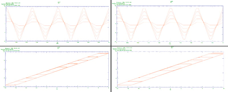
Figure 1. Clockwise from top-left, Figures 1 through 4 from part 1 of this series.
As you can see, it is evident that these hysteresis characteristics cause significant distortion.
A High-Frequency (HF) Signal Example
Consider a large high-frequency sinewave magnetization signal. Even with hysteresis, the average of the recorded signal will be zero. If this signal is now DC offset with another signal, the HF (high-frequency) signal will now, essentially, swing around this offset signal, independent of the deadband as the large signal always drives the magnetization through the deadband. This is true despite the HF signal having waveform distortion.
Thus, the average of the HF bias signal will equal the offset signal, and it is this average value that forms the recorded signal for playback. In this way, the offset signal does not experience the deadband distortion as it would do if it was the only applied signal. The wave shape of the HF bias does not matter so long as its frequency is high enough such that all spurious signals are outside the bandwidth of the desired signal, as they can be filtered out.
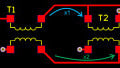
A schematic illustrating this is shown below. The diode and capacitor model the DC hysteresis and non-linear deadband. It is the deadband that causes the distortion.
You'll see how the high-frequency oscillator bias reduces tap recording distortion. Without the HF bias, hysteresis severely distorts the output signal. When the signal changes direction, the output DC magnetization lags the input. However, forcing the input to swing positive and negative overrides the lag and allows the output to depend on the average of the hysteresis curves. The input signal is constructed of two frequencies to show that both THD (total harmonic distortion) and IMD (intermodulation distortion) are eliminated.
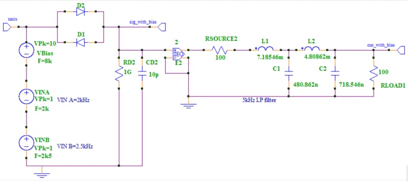
Figure 2. Tape distortion reduction schematic
The schematic shows the sum of three sinewave voltages. Two signals represent a multi-frequency input while the other is the HF bias signal. The two signals illustrate the effect of intermodulation distortion. A nonlinear system will show sum and difference frequencies.
Raw Input/Output Signals
Typical, raw single input/output signals are shown here:
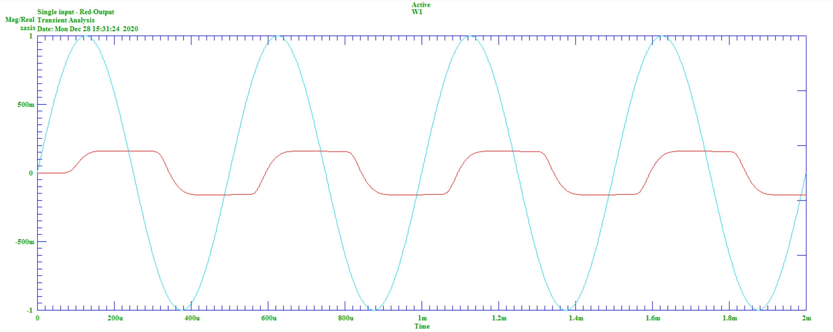
Figure 3. Single-frequency signal, VIN=1V
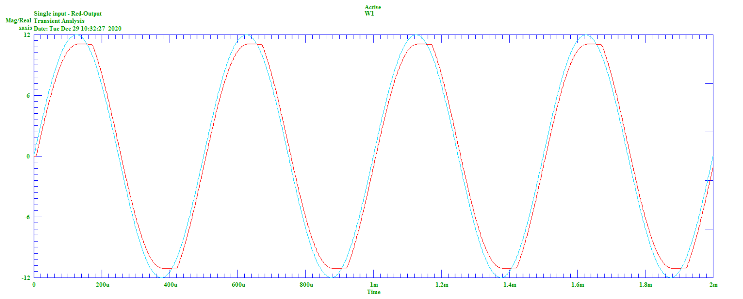
Figure 4. Single-frequency signal, VIN=12V
Figures 3 and 4 show the effective magnetization signal “voltage lagging” its input, and are subsequently severely distorted due to the hysteresis that occurs when the signal changes direction. As we talked about in the last article, a standard SPICE technique that generates a voltage lag would not model this distortion of the waveform peaks.
Mixed Raw Signal
The mixed, raw signal is shown here:
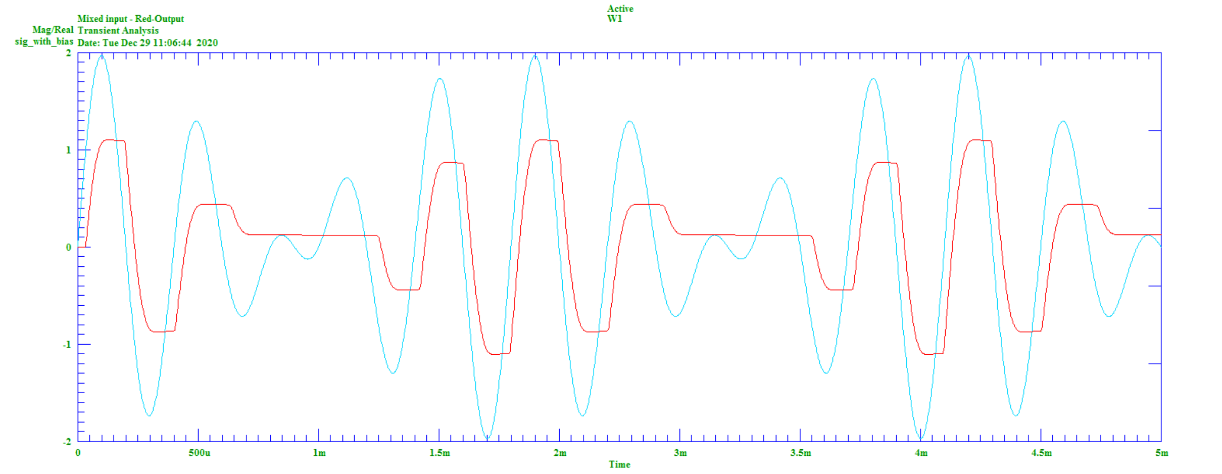
Figure 5. Mixed frequency signal, VINA=1V, VINB=1V
Figure 5 shows that there is significant distortion of the input signal.
FFTs (fast Fourier transforms) of the mixed, unbiased signal are shown here:
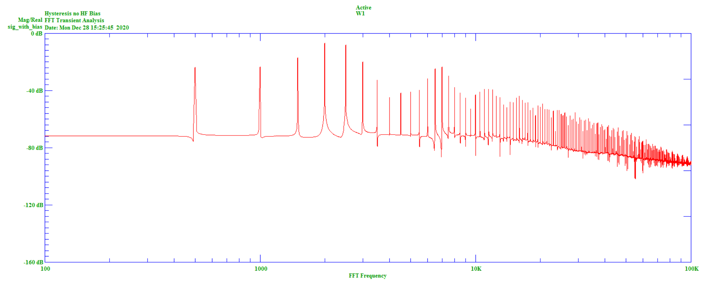
Figure 6. Unbiased mixed-signal FFT VINA=1V, VINB=1V
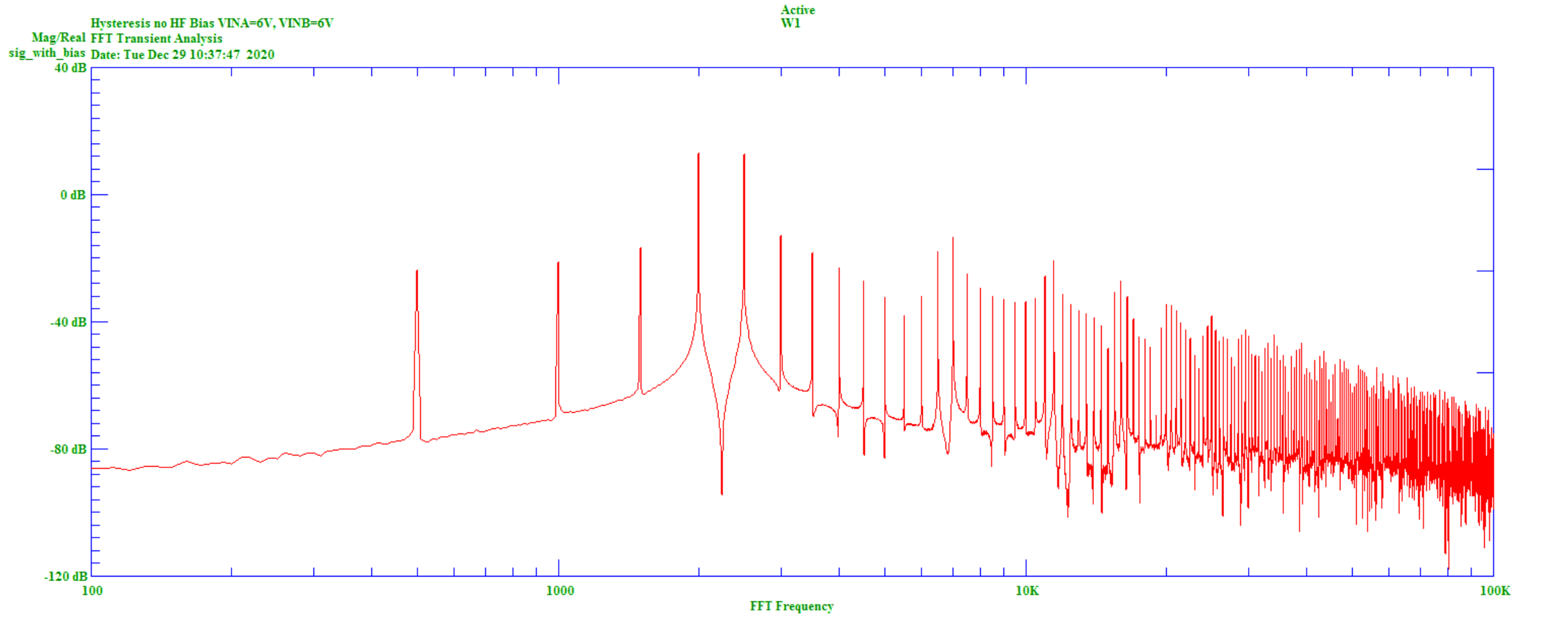
Figure 7. Unbiased mixed-signal FFT, VINA=6V, VINB=6V
These show significant 500 Hz, 1kHz and 1k5 intermodulation distortion for the unbiased condition.
Mixed High-Frequency Signal
The mixed, HF biased signal is shown here:
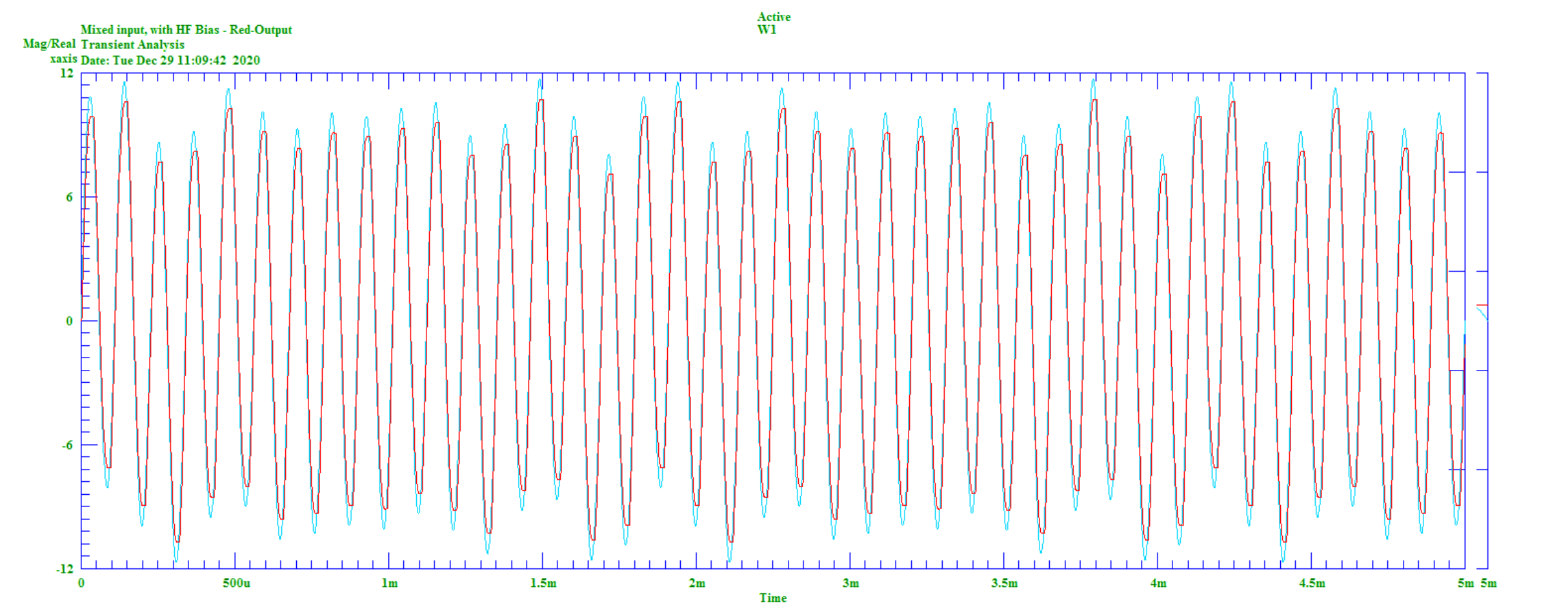
Figure 8. HF biased, mixed signal
The FFT of the mixed, HF biased signal is shown here:
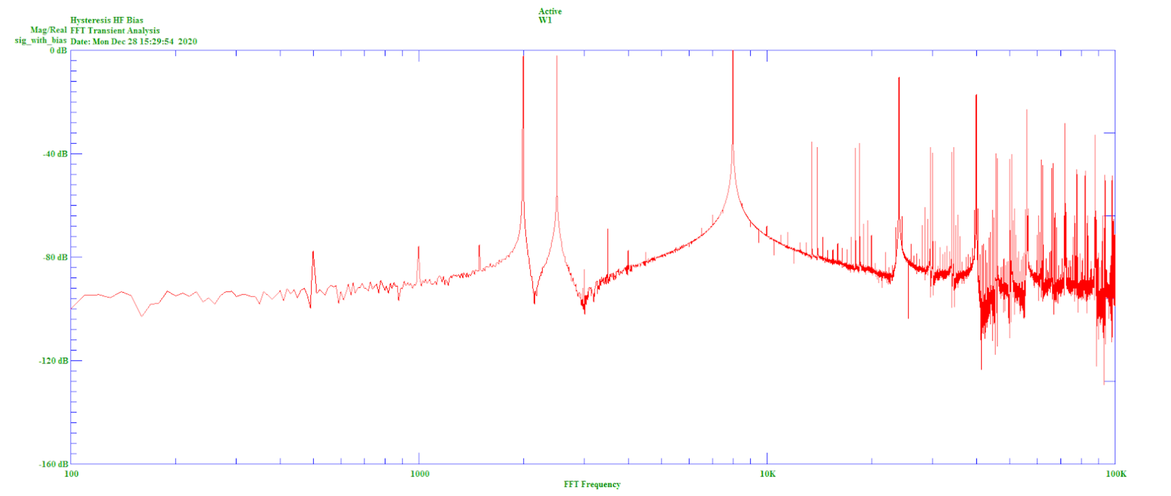
Figure 9. HF biased mixed signal FFT
The addition of the HF bias thus shows greatly reduced intermodulation products.
Summary
This article has demonstrated a technique that allows for the modeling of hysteresis within the capabilities of standard SPICE. This technique may be expanded upon in order to construct inductors with hysteresis, and such a technique will be described in a follow-up article.
Related Content