An Introduction to the Fast Fourier Transform

This article will review the basics of the decimation-in-time FFT algorithms.

The discrete Fourier transform (DFT) is one of the most powerful tools in digital signal processing. The DFT enables us to conveniently analyze and design systems in frequency domain; however, part of the versatility of the DFT arises from the fact that there are efficient algorithms to calculate the DFT of a sequence. A class of these algorithms are called the Fast Fourier Transform (FFT). This article will, first, review the computational complexity of directly calculating the DFT and, then, it will discuss how a class of FFT algorithms, i.e., decimation in time FFT algorithms, significantly reduces the number of calculations.

Computational Complexity of Directly Calculating the DFT

As discussed previously, the N-point DFT equation for a finite-duration sequence, $$x(n)$$, is given by

 

$$X(k)=\sum\limits_{n=0}^{N-1}{x(n){{e}^{-j\tfrac{2\pi }{N}kn}}}$$

Equation 1

 

Let’s see how many multiplications and additions are required to calculate the DFT of a sequence using the above equation. For each DFT coefficient, $$X(k)$$, we should calculate $$N$$ terms including $$x(0){{e}^{-j\tfrac{2\pi }{N}k \times 0}}$$, $$x(1){{e}^{-j\tfrac{2\pi }{N}k \times 1}}$$, ..., $$x(N-1){{e}^{-j\tfrac{2\pi }{N}k \times (N-1)}}$$ and then, calculate the summation. $$x(n)$$ is a complex number in general, and, hence, each DFT output needs approximately $$N$$ complex multiplications and $$N-1$$ complex additions. A single complex multiplication itself requires four real multiplications and two real additions. This can be simply verified by considering the multiplication of $$d_1=a_1+jb_1$$ by $$d_2=a_2+jb_2$$, which leads to 

 

$$d_1d_2=(a_1a_2-b_1b_2)+j(b_1a_2+a_1b_2)$$

 

Moreover, a complex addition itself requires two real additions. Therefore, each DFT coefficient requires $$4N$$ real multiplications and $$2N+2(N-1)=4N-2$$ real additions. To have all the DFT coefficients, we have to compute Equation 1 for all $$N$$ values of $$k$$, therefore an N-point DFT analysis requires $$4N^2$$ real multiplications and $$N(4N-2)$$ real additions. The important point is that the number of calculations of an N-point DFT is proportional to $$N^2$$ and this can rapidly increase with $$N$$. Figure 1 plots the number of real multiplications versus the DFT length $$N$$. Several algorithms are developed to alleviate this problem. In the following section, we will derive one of the basic algorithms of calculating the DFT.

 

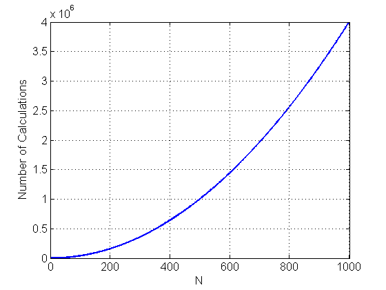
Figure 1. The number of real multiplications for an N-point DFT.

Decimation-in-Time FFT Algorithms

The main idea of FFT algorithms is to decompose an N-point DFT into transformations of smaller length. For example, if we devise a hypothetical algorithm which can decompose a 1024-point DFT into two 512-point DFTs, we can reduce the number of  real multiplications from $$4,194,304$$ to $$2,097,152$$. This is an improvement by a factor of two. In the rest of this article, we will review one of these algorithms which is called the decimation-in-time FFT algorithm.

Let’s see how we can reformulate an N-point DFT in terms of DFTs of smaller length. To have a better insight into the algorithm, we will explain the procedure through examining an eight-point DFT as an example.

Investigation of an Eight-Point DFT

Assume that $$x(n)$$ is a sequence of length eight. Using Equation 1, we can find the eight-point DFT of $$x(n)$$ as

 

$$X\left(k\right)=x(0){{e}^{-j\tfrac{2\pi }{8}k\times0}}+x(1){{e}^{-j\tfrac{2\pi }{8}k\times1}}+x(2){{e}^{-j\tfrac{2\pi }{8}k\times2}}+\dots +x(7){{e}^{-j\tfrac{2\pi }{8}k\times7}}$$

Equation 2

 

Our goal is to examine the possibility of rewriting this eight-point DFT in terms of two DFTs of smaller length. We see that the length of the DFT, $$N=8$$ in this case, appears as the denominator in the complex exponentials. This leads us to the idea that what if we choose and group some terms of Equation 2 in a way that allows us to simplify the fractions $$-\tfrac{j2\pi}{8}kn$$. In this way, we may extract a DFT of smaller length out of Equation 2. For example, since in our case $$N$$ is an even number, we examine choosing all the terms with an even sample index, i.e., $$x(0)$$, $$x(2)$$, $$x(4)$$, and $$x(6)$$. Hence, we have

 

$$G\left(k\right)=x(0){{e}^{-j\tfrac{2\pi }{8}k\times0}}+x(2){{e}^{-j\tfrac{2\pi }{8}k\times2}}+x(4){{e}^{-j\tfrac{2\pi }{8}k\times4}}+x(6){{e}^{-j\tfrac{2\pi }{8}k\times6}}$$

Equation 3

 

After simplifying the fractions in the complex exponentials, we obtain

 

$$G\left(k\right)=x(0){{e}^{-j\tfrac{2\pi }{4}k\times0}}+x(2){{e}^{-j\tfrac{2\pi }{4}k\times1}}+x(4){{e}^{-j\tfrac{2\pi }{4}k\times2}}+x(6){{e}^{-j\tfrac{2\pi }{4}k\times3}}$$

Equation 4

 

Comparing Equation 4 with Equation 1, we observe that $$G(k)$$ is the four-point DFT of $$x(0)$$, $$x(2)$$, $$x(4)$$, and $$x(6)$$. So far, we have shown that half of the computations in Equation 2 can be replaced with a four-point DFT. But how can we simplify the rest of the calculations. The remaining terms, which correspond to odd-index samples, are given by

 

$$H_{1}\left(k\right)=x(1){{e}^{-j\tfrac{2\pi }{8}k\times1}}+x(3){{e}^{-j\tfrac{2\pi }{8}k\times3}}+x(5){{e}^{-j\tfrac{2\pi }{8}k\times5}}+x(7){{e}^{-j\tfrac{2\pi }{8}k\times7}}$$

Equation 5

To simplify the fractions $$-\tfrac{j2\pi}{8}kn$$, we can simply factor $$e^{-j\tfrac{2\pi}{8}k}$$ and obtain

 

$$H_{1}\left(k\right)= {{e}^{-j\tfrac{2\pi }{8}k\times1}}\left( x(1){{e}^{-j\tfrac{2\pi }{8}k\times0}}+x(3){{e}^{-j\tfrac{2\pi }{8}k\times2}}+x(5){{e}^{-j\tfrac{2\pi }{8}k\times4}}+x(7){{e}^{-j\tfrac{2\pi }{8}k\times6}} \right)$$

Equation 6

 

Hence, we have

 

$$H_{1}\left(k\right)= {{e}^{-j\tfrac{2\pi }{8}k\times1}}\left( x(1){{e}^{-j\tfrac{2\pi }{4}k\times0}}+x(3){{e}^{-j\tfrac{2\pi }{4}k\times1}}+x(5){{e}^{-j\tfrac{2\pi }{4}k\times2}}+x(7){{e}^{-j\tfrac{2\pi }{4}k\times3}} \right)$$

Equation 7

 

Again comparing with Equation 1, we observe that $$H_{1}(k)$$ is obtained by multiplying $$e^{-\tfrac{j2\pi}{8}k}$$ by the four-point DFT of $$x(1)$$, $$x(3)$$, $$x(5)$$, and $$x(7)$$. Hence, we have achieved the goal of decomposing an eight-point DFT into two four-point ones. Defining

 

$$H\left(k\right)= x(1){{e}^{-j\tfrac{2\pi }{4}k\times0}}+x(3){{e}^{-j\tfrac{2\pi }{4}k\times1}}+x(5){{e}^{-j\tfrac{2\pi }{4}k\times2}}+x(7){{e}^{-j\tfrac{2\pi }{4}k\times3}}$$

Equation 8

We get the final result as

 

$$X\left(k\right)=G\left(k\right)+{{e}^{-j\tfrac{2\pi }{8}k\times1}}H\left(k\right)$$

Equation 9

 

where $$G(k)$$ and $$H(k)$$ correspond to four-point DFTs. We will soon discuss the flow graph of the above decomposition but there is one subtle point unexplained: How the above procedure can reduce the number of multiplications while $$G(k)+e^{-\tfrac{j2\pi}{8}k \times 1}H(k)$$ requires almost the same number of multiplications as $$X(k)$$ in Equation 2 does. We have only rearranged the terms and changed the coefficients of the multiplications but we have not omitted any multiplication. To resolve this apparent contradiction, we should note three points: firstly, a discrete complex exponential, $$e^{-\tfrac{j2\pi}{N}kn}$$, is a periodic function of $$k$$ with period N. Secondly, the range of $$k$$ in our discussion is from $$0$$ to $$7$$. Thirdly, while Equation 2 is in terms of complex exponentials with period $$8$$, i.e., $$e^{-j\tfrac{2\pi}{8}kn}$$, Equation 9 is basically in terms of four-point DFTs, $$G(k)$$ and $$H(k)$$, which are summations of complex exponentials with period $$4$$. This periodic behavior allows us to reduce the overall computational complexity when computing all of the DFT coefficients. For example, when calculating both $$X(k)$$ and $$X(k+4)$$, we have to evaluate the terms of Equation 2 twice; however, based on Equation 9, we obtain the following equations:

$$X\left(k\right)=G\left(k\right)+{{e}^{-j\tfrac{2\pi }{8}k\times1}}H\left(k\right)$$

Equation 10

 

and 

 

$$X\left(k+4\right)=G\left(k+4\right)+{{e}^{-j\tfrac{2\pi }{8}(k+4)\times1}}H\left(k+4\right)$$

Equation 11

 

Since $$G(k)$$ and $$H(k)$$ are periodic with $$4$$, Equation 11 gives

 

$$X\left(k+4 \right)=G\left(k\right)+{{e}^{-j\tfrac{2\pi }{8}\left (k+4 \right) \times1}}H\left(k\right)$$

Equation 12

 

Comparing Equation 12 with Equation 10 clarifies how breaking an eight-point DFT into two four-point DFTs allows us to use almost the same computations for both $$X(k)$$ and $$X(k+4)$$ and significantly decrease the number of calculations through the periodicity property.

Figure 2 uses the above discussion to obtain the flow graph of decomposing an eight-point DFT into two four-point ones. Note that, in this figure, $$N=8$$ and $$W_{N}^{k}=e^{-j\tfrac{2\pi}{N}k}$$.

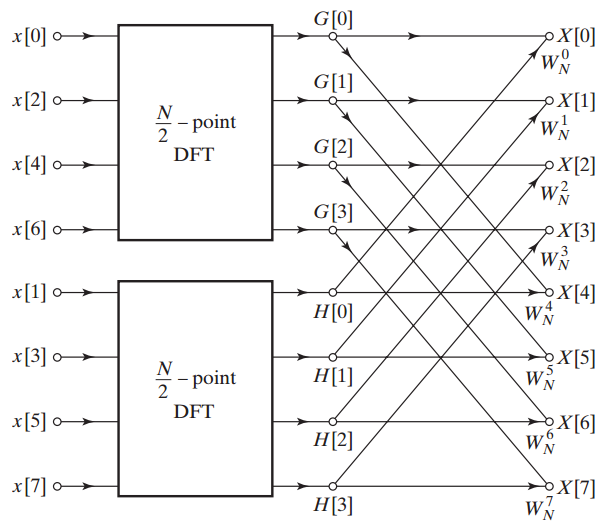
Figure 2. The flow graph of breaking an eight-point DFT into two four-point ones. Image courtesy of Discrete-Time Signal Processing.

While, using the definition of the DFT, we need to perform $$4N^2=256$$ real multiplications for an eight-point DFT, the discussed algorithm needs to perform two four-point DFTs along with $$N$$ complex multiplications (see Figure 2). For the two four-point DFTs we need to perform a total of $$2\times 4 \times (\tfrac{N}{2})^2=2\times 4 \times 4^2=128$$ real multiplications. The $$N$$ extra complex multiplications require $$4N=4 \times 8=32$$ real multiplications. Hence, the above algorithm needs a total of $$160$$ real multiplications which is much smaller than that of the direct computation method.

This is a considerable improvement but can we achieve further simplification by applying the discussed method to the four-point DFTs of Figure 2? We saw that the starting point of the algorithm was that the DFT length N was even and we were able to simplify the complex exponentials of even index samples. Hence, to apply the algorithm one more time, we need $$\tfrac{N}{2}$$ to be divisible by 2. In this particular example, $$\tfrac{N}{2}=4$$ and following a procedure similar to the above discussion we can decompose each of the four-point DFTs into two two-point ones. For example, the upper $$\tfrac{N}{2}$$-point DFT of Figure 2 can be replaced by the flow graph of Figure 3.

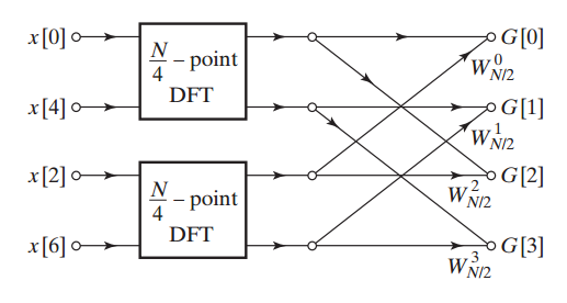
Figure 3. The flow graph of breaking a four-point DFT into two two-point ones. Image courtesy of Discrete-Time Signal Processing.

Substituting the four-point DFTs of Figure 2 with the flow graph given in Figure 3, we obtain the structure in Figure 4. Note that Figure 4 replaces $$W_{\tfrac{N}{2}}$$ coefficients of Figure 3 with $$W_{N}^{2}$$ because $$e^{-j\tfrac{2\pi}{(\tfrac{N}{2})}}=e^{-j\tfrac{2\pi}{N} \times 2}$$.

 

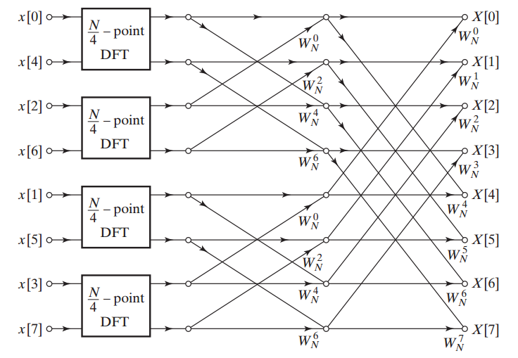
Figure 4. The flow graph to calculate an eight-point DFT using four two-point ones. Image courtesy of Discrete-Time Signal Processing.

Finally, we can replace the two-point DFTs of Figure 4 with the flow graph given in Figure 5 and obtain the final structure given by Figure 6.

 

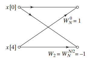
Figure 5. The flow graph used to compute the uppermost two-point DFT of Figure 4. Image courtesy of Discrete-Time Signal Processing.

 

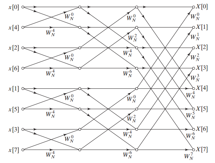
Figure 6. The decimation-in-time based structure to compute an eight-point DFT. Image courtesy of Discrete-Time Signal Processing.

The discussed example shows that in order to repeatedly apply this technique until we are left with two-point DFTs, we have to choose the length of the original DFT to be a power of two, i.e., $$N=2^{\nu}$$. In this case, after $$log_{2}(N)$$ iterations, we will reach two-point DFTs. As Figure 6 suggests each stage of the algorithm requires N complex multiplications and hence, the total number of complex multiplications will be $$Nlog_{2}(N)$$. In the example of the eight-point DFT, we will have $$8log_{2}(8)=24$$ complex multiplications. Then, while the direct computation of the eight-point DFT requires $$256$$ real multiplications, the decimation-in-time method requires only $$24 \times 4=96$$ real multiplications. The reader can easily verify that the computational saving will be really dramatic for large DFTs.

 

As a final note, remember that it is still possible to utilize the symmetry and the periodicity of the complex coefficients of Figure 6, and reduce the number of complex multiplications by a factor of two. For a detailed explanation of this simplification see page 729 of this book.