Second-Order Type-2 PLLs: Bode Diagrams, Bandwidth, and Overshoot

Learn how to select the zero frequency, damping factor, and loop bandwidth for one of the most popular PLL configurations.

Technical Article February 08, 2026 by Dr. Steve Arar

Previously, we learned that a Type-2 PLL offers superior performance regarding steady-state phase error when compared to a Type-1 PLL. Since nearly all practical PLLs are either second-order or can be approximated as second-order loops, this article will focus on second-order Type-2 PLLs. By examining their Bode plots, we'll develop simple design equations that help us choose important loop parameters.

Since the second-order Type-2 PLL can be understood as a special case of the second-order PLL with a lag-lead filter, we'll start by reviewing the Bode plots of the latter configuration. At the end of the article, we'll also examine the closed-loop bandwidth and peak overshoot of the Type-2 PLL.

Bode Plots of the PLL With a Lag-Lead Filter

The linear model of a basic PLL is shown in Figure 1.

Linear model of a basic PLL.

Figure 1. Linear model of a basic PLL.

The transfer function of the lag-lead loop filter may be described by:

$$G(s) ~=~ \frac{1~+~ s / \omega_z}{1~+~ s / \omega_p}$$

Equation 1.

where ω_z and ω_p denote the zero and pole frequency, respectively. Hence, for a second-order PLL with a lag-lead filter, the open-loop transfer function is:

$$F(s) ~=~ \frac{K_0}{s} ~\times~ \frac{1~+~ s / \omega_z}{1~+~ s / \omega_p}$$

Equation 2.

Figure 2 shows the Bode magnitude plot of this transfer function. Its key characteristics are highlighted in orange.

The magnitude plot of a PLL with a lag-lead loop filter.

Figure 2. The magnitude plot of a PLL with a lag-lead loop filter.

At low frequencies, the integration action of the VCO results in an asymptotic amplitude slope of –20 dB/decade. The pole of the loop filter introduces a breakpoint, resulting in a slope of –40 dB/decade. Another breakpoint is introduced by the zero, changing the slope from –40 to –20 dB/decade.

The low-frequency region of the magnitude plot with a –20 dB/decade slope corresponds to the term K₀/jω from the open-loop transfer function, F(s), shown in Equation 2. Consequently, the extension of this line intersects the unity-gain axis at ω = K₀, as illustrated in the above figure.

It can be shown that the extension of the line with a –40 dB/decade slope intersects the horizontal axis at the loop natural frequency (ω_n).

The slope of the line going through ω_n is twice the slope of the line going through ω = K₀. Therefore, ω_n is the midpoint between ω_p and K₀ on a logarithmic plot. This observation results in the following equation:

$$\omega_n^2 ~=~ \omega_p K_0$$

Equation 3.

Similarly, ω_n is also positioned midway between ω_z and the gain crossover frequency (ω_c) on a logarithmic plot. This results in the following expression:

$$\omega_n^2 ~=~ \omega_z \omega_c$$

Equation 4.

Combining Equations 3 and 4, we can express the gain crossover frequency in terms of the pole and zero frequencies:

$$\omega_c ~=~ K_0 \frac{\omega_p}{\omega_z}$$

Equation 5.

Now that we've completed our review, let's examine the Bode diagram of the second-order Type-2 configuration.

Bode Magnitude Plot of Second-Order Type-2 PLLs

The basic second-order Type-2 PLL uses the following loop filter:

$$G(s) ~=~ \frac{1 ~+~ s/\omega_z}{s}$$

Equation 6.

leading to the open-loop transfer function:

$$F(s) ~=~ \frac{K_0}{s^2} ~\times~ (1~+~ s / \omega_z)$$

Equation 7.

In this case, the loop filter has a pole at the origin.

By comparing Equation 7 with Equation 2, we see that a second-order Type-2 PLL resembles a PLL with a lag-lead filter, assuming the pole is designed to be very close to the origin. For frequencies well above the pole frequency (ω_p), the open-loop transfer function of the PLL with a lag-lead filter (Equation 2) can be approximated as:

$$F(s) ~=~ \frac{K_0}{s^2} ~\times~ (1~+~ s / \omega_z)$$

Equation 8.

which, aside from a multiplicative factor, is identical to Equation 7 for a Type-2 PLL.

We now use Equation 7 to obtain the Bode magnitude plot (Figure 3).

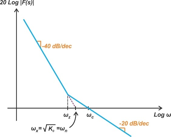
The open-loop magnitude plot of the second-order Type-2 PLL.

Figure 3. The open-loop magnitude plot of the second-order Type-2 PLL.

Since the open-loop transfer function contains two poles at the origin, the asymptotic amplitude slope at low frequencies is –40 dB/decade. The zero of the loop filter introduces a breakpoint, changing the slope from –40 to –20 dB/decade.

The low-frequency region of the magnitude plot corresponds to the term K₀/ω² from the Type-2 PLL's open-loop transfer function. As illustrated in the above figure, the extension of this line intersects the horizontal axis at ω_x = √K₀. Note that the horizontal axis corresponds to 0 dB, or unity gain.

Please be aware that while K₀ has units of rad/s in the PLL model featuring a lag-lead filter, in the Type-2 PLL model, it takes on units of (rad/s)², making its square root a frequency.

Identifying the Natural Frequency in the Bode Plot

The closed-loop transfer function of the Type-2 PLL is shown below:

$$H(s) ~=~ \frac{\phi_{vco}}{\phi_{in}} (s) ~=~ \frac{K_0(1 ~+~ s/\omega_z)}{s^2~+~K_0s/ \omega_z~+~K_0}$$

Equation 9.

Comparing the denominator with the standard control theory form (s² + 2ζω_ns + ω_n²) we see that the loop natural frequency is:

$$\omega_n ~=~ \sqrt{K_0}$$

Equation 10.

and the damping factor is:

$$\zeta ~=~ \frac{\sqrt{K_0}}{2 \omega_z}$$

Equation 11.

Comparing Equation 10 with the expression obtained for ω_x in the previous section, we see that the extension of the low-frequency region of the magnitude plot intersects with the horizontal axis at the loop natural frequency (ω_x = ω_n).

Estimating Crossover Frequency

Referring to Figure 3, the slope of the line going through ω_n is twice the slope of the line going through the gain crossover frequency (ω_c). Consequently, ω_n is at the midpoint between ω_z and ω_c on a logarithmic plot, leading to the following equation:

$$\omega_n^2 ~=~ \omega_z \omega_c$$

Equation 12.

Note that this relationship is valid for both the Type-2 PLL and the PLL with a lag-lead filter (see Equation 4).

Combining Equations 12 and 10, we can express the crossover frequency in terms of K₀ and ω_z:

$$\omega_c ~=~ \frac{K_0}{\omega_z}$$

Equation 13.

Example 1: Determining Zero Frequency and Damping Factor for Type-2 PLL

A Type-2 PLL is to be designed to have a phase margin of PM = 76 degrees. If the loop gain is K₀ = 2.09 × 10⁵ (rad/s)², find the zero frequency (ω_z) and the damping factor (ζ).

Solution

The phase of the open-loop transfer function is –180 degrees, contributed by the two poles at the origin, plus the phase contributed by the zero. At the gain crossover frequency, the phase is:

$$Phase ~=~ -180~ \text{degrees} ~+~ \tan^{-1}(\frac{\omega_c}{\omega_z})$$

Equation 14.

Adding 180 degrees to the above equation yields the phase margin:

$$PM ~=~ \tan^{-1}(\frac{\omega_c}{\omega_z})$$

Equation 15.

For a phase margin of PM = 76 degrees, we should have ω_c = 4ω_z, meaning that the crossover frequency is four times the zero frequency. The damping factor can be determined from the ratio of ω_c to ω_z, even without information about the loop gain. To do so, we first combine Equations 10 and 11 to obtain:

$$\zeta ~=~ \frac{\omega_n}{2 \omega_z}$$

Equation 16.

Substituting ω_n from Equation 12 into the above equation, we have:

$$\zeta ~=~ \frac{1}{2} \sqrt{\frac{\omega_c}{\omega_z}}$$

Equation 17.

Now, assuming that ω_c = 4ω_z, the damping factor works out to ζ = 1. To find the zero frequency, we substitute ω_c = 4ω_z and K₀ = 2.09 × 10⁵ (rad/s)² into Equation 13, producing:

$$\omega_z ~=~ \frac{1}{2} \sqrt{K_0}~=~ \frac{1}{2} \sqrt{2.09 ~\times~ 10^5}~=~228.58 ~ \text{rad/s}$$

Equation 18.

To verify our calculations, we substitute K₀ = 2.09 × 10⁵ (rad/s)² and ω_z = 228.58 rad/s in the open-loop transfer function equation (Equation 7) and use Matlab to plot the Bode diagrams. These are presented in Figure 4.

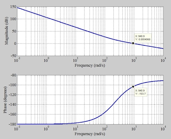
The Bode plots of the open-loop transfer function.

Figure 4. The Bode plots of the open-loop transfer function.

As observed, the crossover frequency is 941 rad/s. This is close to what we would obtain based on our simplified analysis above:

$$\omega_c~=~4 \omega_z~=~4~\times~228.58~=~914~\text{rad/s}$$

Equation 19.

The phase margin from the Matlab plots is PM = 180 – 103.7 = 76.3 degrees, which agrees well with our calculations. If we revise the previous example for a more aggressive design featuring a phase margin of PM = 65 degrees, we arrive at ω_c = 2.14ω_z and ζ = 0.73.

Now that we've discussed the Bode diagrams of the Type-2 PLL, let's learn how to determine its 3-dB bandwidth and overshoot.

Closed-Loop Bandwidth

It can be shown that the closed-loop 3-dB bandwidth of the second-order Type-2 PLL is given by:

$$BW ~=~ \sqrt{K_0 \big ( 1~+~2 \zeta^2 ~+~ \sqrt{2 ~+~ 4 \zeta^2 ~+~ 4 \zeta^4} \big )}$$

Equation 20.

To illustrate how the bandwidth changes with the damping factor, Figure 5 uses the above expression to plot BW/√K₀ against ζ.

Normalized closed-loop bandwidth of the Type-2 PLL vs. the damping factor.

Figure 5. Normalized closed-loop bandwidth of the Type-2 PLL vs. the damping factor.

Note that the square root of K₀ is equal to the natural frequency. The above curve therefore shows how the 3-dB bandwidth normalized to ω_n changes with ζ.

You may be wondering why increasing ζ results in a larger 3-dB bandwidth. To understand this, consider Equation 11. According to this equation, increasing ζ requires either an increase in the loop gain (K₀) or a decrease in the zero frequency (ω_z). As indicated in Equation 13, these adjustments lead to a higher open-loop crossover frequency.

To grasp this trend more effectively, I encourage you to analyze the curve shown in Figure 3. Since the crossover frequency can be interpreted as an estimate of the closed-loop 3-dB bandwidth, you will see that increasing ζ leads to a wider bandwidth.

Peak Overshoot

Another important characteristic of the second-order Type-2 PLL is its peak overshoot in the time domain. Figure 6 illustrates the peak overshoot of this configuration for a unit step change in the input phase.

Overshoot of the Type-2 PLL in response to a unit phase step as a function of the damping factor.

Figure 6. Overshoot of the Type-2 PLL in response to a unit phase step as a function of ζ.

As expected, the overshoot decreases as we increase the damping factor.

Example 2: Finding the Bandwidth and Overshoot of a Type-2 PLL

The PLL designed in the previous example had the following characteristics:

A loop gain of K₀ = 2.09×10⁵ (rad/s)²
A zero frequency of ω_z = 228.58 rad/s
A damping factor of ζ = 1.

Refer to Figures 5 and 6 to determine the 3-dB bandwidth and overshoot of this PLL. Then, compare these results with the responses generated by Matlab.

Solution

With ζ = 1, we expect a normalized 3-dB bandwidth of 2.48, producing:

$$BW / \sqrt{K_0} ~=~ 2.48 ~\quad \Rightarrow \quad BW ~=~ 2.48 ~\times~ \sqrt{2.09 ~\times~ 10^{5}} ~=~ 1133.8 \ \text{rad/s}$$

Equation 21.

This is consistent with the closed-loop magnitude plot of the PLL shown in Figure 7.

Closed-loop magnitude plot of the PLL in our design example.

Figure 7. The closed-loop magnitude plot of the PLL in our design example.

Figure 6 does not indicate the overshoot for ζ = 1. However, given that the overshoot is nearly 15% for ζ values just below unity, we anticipate a comparable overshoot at ζ = 1. Figure 8 shows the Matlab-generated step response of the PLL.

Step response of the PLL in the design example.

Figure 8. The step response of the PLL in our design example.

As observed, the overshoot is 13%, which is reasonably close to that obtained from Figure 6.

Wrapping Up

In practice, second-order Type-2 PLLs are among the most widely utilized PLL configurations. In light of their popularity, this article analyzed their Bode plots to derive straightforward design equations. These equations assist in selecting loop parameters such as the zero frequency, damping factor, and loop bandwidth. We also explored the closed-loop bandwidth and peak overshoot of this PLL configuration.

This article concludes our examination of the loop filter's impact on PLL performance at the system level. In the next article, we'll begin a new series that investigates the loop components at the circuit level, starting with the phase detector.

This article is Part 12 of a 12-part series on loop filters in PLL design. All articles in this series are listed below in order of publication: