Facebook
 Google
 GitHub
 Linkedin
Introducing the Lag-Lead Filter
Learn how using a pole-zero loop filter improves PLL performance and design flexibility over the simpler lag filter.
In the previous articles of this series, we explored first-order PLLs that lack a loop filter and second-order PLLs featuring a lag filter. We then compared these two configurations by working through a design problem using each setup. Through this comparative analysis, we revealed the constraints associated with the lag filter approach.
In this article, we'll introduce a more complex PLL configuration that utilizes a pole-zero loop filter, also known as the lag-lead filter. As the first of these names suggests, it features both a pole and a zero. The filter's transfer function is given by:
$$G(s) ~=~ \frac{1~+~ s / \omega_z}{1~+~ s / \omega_p}$$
Equation 1.
where ωp is the pole frequency and ωz is the zero frequency. We'll examine two distinct scenarios:
- A pole frequency lower than the zero frequency (ωp < ωz).
- A zero frequency lower than the pole frequency (ωz < ωp).
Pole-Zero Filter With ωp < ωz
As an example of the first scenario, let's set ωp = 1 rad/s and ωz = 10 rad/s. The corresponding Bode diagram for G(s) is shown in Figure 1.

Figure 1. The Bode plots of G(s) for ωp = 1 rad/s and ωz = 10 rad/s.
Like the lag filter we discussed previously, the filter defined by Equation 1 exhibits a lowpass characteristic when ωp < ωz. However, the lag filter includes only a pole, resulting in an undesirable phase lag at high frequencies. The lag-lead filter described by Figure 1 features a zero positioned above the pole frequency. This zero contributes a positive phase shift, thereby reducing the overall phase lag introduced by the filter.
As illustrated in Figure 1, at frequencies significantly above the zero frequency, the phase shift approaches zero. Thus, if the zero frequency is sufficiently lower than the open-loop gain crossover frequency, the new filter can achieve a lowpass magnitude characteristic without adding extra phase lag to the loop. To appreciate the benefits of this filter, it's important to remember that excessive phase lag in the loop decreases the phase margin, which in turn makes the system less stable.
A drawback of the lag-lead filter is that its filtering behavior is limited and reaches 20log(ωp/ωz) at high frequencies, whereas the lag filter ideally maintains a roll-off of –20 dB per decade as frequency increases. In other words, the more complex filter offers relatively limited attenuation of higher frequency components.
Pole-Zero Filter With ωp > ωz
To explore the second scenario, let's assume that ωz = 1 rad/s and ωp = 10 rad/s. The corresponding Bode diagram for G(s) is shown in Figure 2.

Figure 2. The Bode plots of G(s) for ωz = 1 rad/s and ωp = 10 rad/s.
In control theory, the pole-zero filter with ωp > ωz is commonly referred to as a lead compensator. In the context of control theory, we generally position the open-loop gain crossover frequency between the pole and zero frequency of a lead compensator. This introduces a positive phase to the open-loop transfer function at the gain crossover frequency, enhancing the stability of the loop. For instance, the phase plot of Figure 2 shows that this particular filter can introduce a maximum positive phase of roughly 55 degrees to the loop.
Although the lag-lead filter with ωp > ωz is a standard compensation method in control theory, using it alone as the loop filter in PLL applications doesn't yield significant benefits. When ωp > ωz, the filter behaves like a highpass filter, making it ineffective at attenuating the undesired components produced by the phase detector.
Wrapping Up
In the previous article, we compared the performance of a first-order PLL with no loop filter to that of a second-order PLL with a lag filter. Our analysis found that the lag filter effectively eliminated undesirable components from the phase detector and provided some control over the loop's response. However, stability concerns left us with limited flexibility in choosing the damping factor. As a result, we achieved only minimal improvements in loop performance and the independent adjustment of parameters.
In this article, we introduced a second-order PLL that uses a more sophisticated filter: the pole-zero filter, also known as the lag-lead filter. This setup incorporates both a pole and a zero, usually with the pole positioned at a lower frequency than the zero.
Compared to using a lag filter, the lag-lead configuration provides increased flexibility in independently choosing parameters such as the loop gain and bandwidth. In the next article, we'll explore the PLL with a lag-lead filter in greater detail.
This article is Part 8 of a 12-part series on loop filters in PLL design. All articles in this series are listed below in order of publication:
- Foundations for PLL Nonlinear Analysis: Modeling the Phase Detector and VCO
- Analyzing a First-Order PLL in Acquisition Mode With a Nonlinear Model
- Analyzing First-Order PLLs Using Linear Models
- Understanding the Limitations of the First-Order PLL
- Introduction to Second-Order Type-1 PLLs
- Understanding the Limitations of the Second-Order Type-1 PLL With a Lag Filter
- Analyzing the Lag Filter’s Effect on PLL Performance
- Introducing the Lag-Lead Filter
- Exploring the Bode Plots of PLLs With a Lag-Lead Loop Filter
- Understanding the Time-Domain Response of PLLs With Lag-Lead Filters
- Introduction to Second-Order Type-2 PLLs
- Second-Order Type-2 PLLs: Bode Diagrams, Bandwidth, and Overshoot
All images used courtesy of Steve Arar