Facebook
 Google
 GitHub
 Linkedin
Practical FIR Filter Design: Part 2 - Implementing Your Filter
Implementing a FIR filter designed in Octave or Matlab on an N-bit microprocessor
In Part 1 we focused on designing a digital filter in Octave/Matlab. This tutorial will outline the steps necessary to implement your filter in actual hardware.
For reference, the code from Part 1 is listed below:
close all;
clear all;
clf;
f1 = 11200;
f2 = 15000;
delta_f = f2-f1;
Fs = 192000;
dB = 30;
N = dB*Fs/(22*delta_f);
f = [f1 ]/(Fs/2)
hc = fir1(round(N)-1, f,'low')
figure
plot((-0.5:1/4096:0.5-1/4096)*Fs,20*log10(abs(fftshift(fft(hc,4096)))))
axis([0 20000 -60 20])
title('Filter Frequency Response')
grid onFrom the code, we obtain the filter coefficients. This is variable 'hc'. We can take a look at the impulse response of the filter by plotting the variable 'hc':
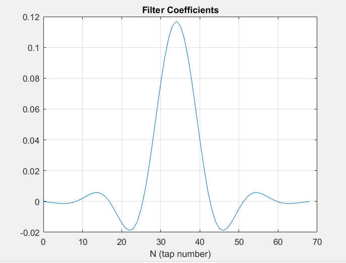
FIGURE 1
Assuming some prior knowledge of DSP, recall that in processing an FIR, it has the topology of Figure 2 below. The impulse response is just the coefficients of the filter. Imagine passing a signal of one time sample duration with a magnitude of 1 into x[n]. The output would simply be that impulse touching each tap ($$b_{n}$$ in Figure 2) producing Figure 1 above.

FIGURE 2
Where:
x[n] - Input signal
$$b_{n}$$ - Nth Coefficient
$$z^{-1}$$ - delay
y[n] - filters output
From Figure 2 we have an idea of how an FIR filter looks in software and hardware. We need to store the coefficients in our microprocessor and pass input through these taps and add them to produce our output. An important step to implementing your coefficients in hardware is quantizing and scaling. When we calculated our coefficients in Octave, we calculated them with high accuracy which is a consequence of the computer used to design them (32-64 bits). When we quantize them for some N-bit processor for implementing them on some hardware, we obtain rounding errors. These rounding errors may affect the time and frequency responses of the digital filter, deviating them from the ideal values.
For the most dramatic example, lets say we want to implement this design on an 8-bit fixed point microprocessor. We need to quantize our coefficients. Lets do this without scaling first. To quantize the coefficients compute the following:
$$h_{quantized} = floor(hc*2^8)/(2^8)$$
Add the following code to compute the quantized coefficients, the quantization error, the quantization error spectrum, and a comparison between the frequency spectrum calculated in Octave and one we would implement on an 8-bit microprocessor.
h_q1 = floor(hc*2^8)/2^8;
q1 = h_q1 - hc;

figure
subplot(211)
plot(q1)
title('Quantization Error')
subplot(212)
plot((-0.5:1/4096:0.5-1/4096)*Fs,20*log10(abs(fftshift(fft(q1,4096)))))
title('Quantization Error Spectrum')

figure
plot((-0.5:1/4096:0.5-1/4096)*Fs,20*log10(abs(fftshift(fft(hc,4096)))))
hold on
plot((-0.5:1/4096:0.5-1/4096)*Fs,20*log10(abs(fftshift(fft(h_q1,4096)))),'color','r')
grid on
axis([-Fs/2 Fs/2 -140 5])
title('Frequency Spectrum - Blue(Octave), Red(8-Bit Quantized)')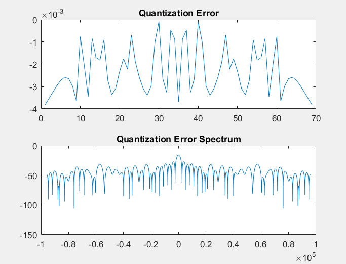
Figure 3
Quantization Error and Quantization Error Spectrum
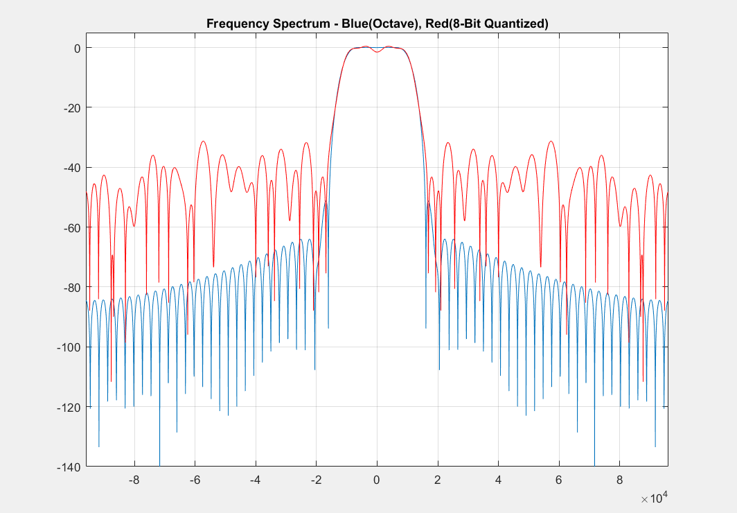
Figure 4
It's easy to see from Figure 4 that the quantization spectrum in red is FAR off from our initial design. The stop band is well above -40dB and the passband has some terrible ripple. This is because our quantization noise shown in Figure 3 has been added to our initial design. In order to tame the response, we need to scale the coefficients. Scaling the coefficients maximizes the range of values the coefficients can take in an actual processing system, which in turn minimizes quantization noise error. We do this as follows:
h_scl = max(hc);
h_q2 = floor((hc/h_scl)*2^8)/2^8;
q2 = h_scl *h_q2 - hc;

h_q2 = h_q2/sum(h_q2);

figure
subplot(211)
plot(q1)
title('Quantization Error')
subplot(212)
plot((-0.5:1/4096:0.5-1/4096)*Fs,20*log10(abs(fftshift(fft(q2,4096)))))
title('Quantization Error Spectrum')

figure
plot((-0.5:1/4096:0.5-1/4096)*Fs,20*log10(abs(fftshift(fft(hc,4096)))))
hold on
plot((-0.5:1/4096:0.5-1/4096)*Fs,20*log10(abs(fftshift(fft(h_q2,4096)))),'color','r')
grid on
axis([-Fs/2 Fs/2 -140 5])
title('Frequency Spectrum W/ Scaling - Blue(Octave), Red(8-Bit Quantized)')
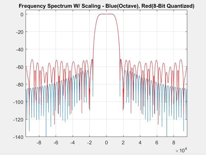
Figure 5
With scaling, we see the frequency spectrum is much better behaved than that of Figure 4. Our stop band matches our intial design of being below -40dB and our passband ripple has been reduced. There is still a fair amount of error associated with this example because we chose to implement this on an 8-bit microprocessor, but scale this up to 16 or higher and you will find that your design almost exactly matches your implementation coefficients.
This tutorial shows the importance of quantization and coefficient scaling for implementing an FIR filter on real hardware.
Related Content