Facebook
 Google
 GitHub
 Linkedin
Design of FIR Filters Using the Frequency Sampling Method
This article will review the basics of the frequency sampling method for designing FIR filters.
This article will review the basics of the frequency sampling method for designing Finite Impulse Response (FIR) filters.
FIR filters have two main advantages over Infinite Impulse Response (IIR) filters:
- An FIR filter has no feedback loop and is inherently stable. (We always need to check the stability of an IIR filter.)
- An FIR filter can easily provide a linear-phase response, which is crucial in phase-sensitive applications such as data communications, seismology, etc.
This article will teach you how to design an FIR filter using the frequency sampling method.
FIR Filter Design by Windowing
Let's assume that we want to design a Finite Impulse Response (FIR) filter with the desired frequency response $$H_{d}(\omega)$$. The window method applies the inverse discrete-time Fourier transform to find the corresponding time-domain representation, $$h_{d}(n)$$, as given by
$$h_{d}(n)=\frac{1}{2\pi}\int_{-\pi}^{\pi}H_{d}(\omega)e^{jn\omega}d\omega$$
Equation 1
Generally, $$h_{d}(n)$$ is not of finite length and since we were looking for a finite impulse response, we can truncate $$h_{d}(n)$$ and achieve an approximation of the desired response. This is equivalent to multiplying $$h_d(n)$$ by a rectangular window.
As discussed in a previous article, From Filter Specs to Window Parameters in FIR Filter Design, we can use other window functions to achieve a trade-off between ripples in the passband and the sharpness of the transition band.
For many classic filters, we can easily calculate the integral of Equation 1. For example, assume that we are designing an ideal lowpass filter with cutoff frequency of $$\omega_c$$. Then, we have
$$H_d(\omega)=\begin{cases}1 & | \omega | \leq \omega_c \\0 & else\end{cases}$$
Equation 2
In this particular example, some mathematical manipulations can easily lead us to the corresponding $$h_d(n)$$ (see Equation (8) in this article) because $$H_d(\omega)$$ is given by a simple equation. Then, we can apply a suitable window function to arrive at a finite-length response which is an approximation of the desired filter. For more details of this discussion, please see this article on FIR filter design by windowing.
However, if $$H_d(\omega)$$ has a complicated equation, we wouldn’t be able to easily calculate Equation 1. In these cases, we can use the frequency sampling method to design FIR filters with an arbitrary $$H_d(\omega)$$.
In this article, we will first review a practical example where the required FIR filter has a complicated frequency response and the frequency sampling method is quite helpful. Then, we will review the basics of FIR filter design using this method.
An FIR Filter to Compensate for the $$\tfrac{sin(x)}{x}$$ Distortion
We can think of a practical DAC as an ideal DAC, which produces an impulse train, followed by a zero-order hold block.
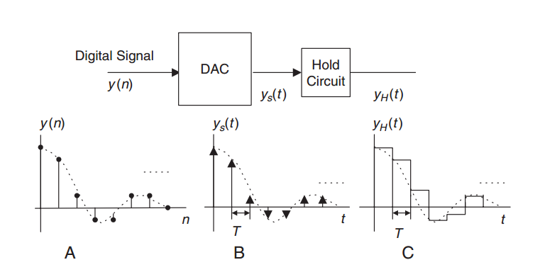
Figure 1. Practical DACs generally apply a zero-order hold to the output values. Image courtesy of Digital Signal Processing.
The hold circuit is required because, in practice, we cannot produce the narrow pulses of an ideal DAC. However, placing a zero-order hold at the output of an ideal DAC (as shown in Figure 1) means that the ideal output, $$y_s(t)$$, will be modified by the transfer function of the hold circuit. It can be shown that the transfer function of the zero-order hold is given by
$$H(f)=t_{h}\frac{sin(\pi f t_{h})}{\pi f t_{h}}$$
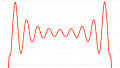
where $$t_h$$ is the hold time which is generally equal to the sampling period. The following figure shows the normalized frequency response of the hold circuit, i.e., $$H_{DAC}=\tfrac{H(f)}{t_h}$$.
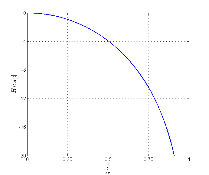
Figure 2. The normalized frequency response of the hold circuit versus $$\tfrac{f}{f_s}$$.
As the above figure shows, the frequency components near $$\tfrac{f_s}{2}$$ experience an attenuation of about $$4$$ dB compared to the low-frequency components. We discussed in a previous article on multirate DSP in D/A conversion that it is possible to employ a multirate system to alleviate the problem. However, for relatively small values of oversampling ratio (e.g., $$L\leq 8$$), we may still need to compensate for the hold circuit distortion. To this end, we can apply a filter with the frequency response of $$\tfrac{1}{H_{DAC}}$$ to $$y(n)$$ in Figure 1.
Assuming that we are using a multirate system (see Figure 3), we can modify the interpolation filter itself to avoid the use of an extra filter. In this case, the magnitude of the interpolation filter response will be proportional to $$\tfrac{1}{H_{DAC}}$$ in the filter passband ($$0 \leq \omega \leq \tfrac{\pi}{L}$$ for an L-fold interpolation) and zero otherwise.

Figure 3. $$H(z)$$ can be designed to both eliminate the frequency components above $$\tfrac{\pi}{L}$$ and compensate for the hold circuit distortion. Image courtesy of Digital Signal Processing.
To summarize, we can use Equation 1 to design ideal filters such as the one given by Equation 2. However, this method is not easy when designing a filter with an arbitrary frequency response, e.g., when designing the magnitude of $$H(z)$$ to be equal to $$\tfrac{1}{H_{DAC}}$$ in a particular band. In these cases, we can use the frequency sampling method.
The Frequency Sampling Method
The frequency sampling method is based on replacing the integral of Equation 1 by an approximate sum. Let's assume that we need to design a filter with the frequency response shown in Figure 4.
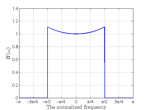
Figure 4. The frequency sampling method can be used to design a filter with an arbitrary frequency response such as $$H(\omega)$$.
To have simpler mathematical expressions, we can approximate $$H(\omega)$$ using the red curve in the following figure.
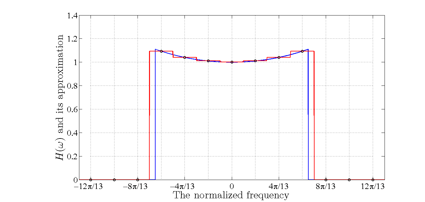
Figure 5. The red curve is an approximation of $$H(\omega)$$.
In this particular example, the desired frequency response is sampled at regular frequency intervals $$\tfrac{2\pi}{13}k$$ for $$k=0, 1, 2, \dots, 12$$ (the samples are shown by dots in the figure). If we were to calculate the integral of $$H(\omega)$$ itself, we could simply approximate the integral calculating the area under the red curve which is sum of $$13$$ rectangles of width $$\tfrac{2\pi}{13}$$ and length determined by the samples of $$H(\omega)$$. To perform the integral of Equation 1, we also need to take the term $$e^{jn\omega}$$ into account. Hence, for $$N=2M+1$$ samples of $$H(\omega)$$, we can approximate Equation 1 using
$$h_{d}(n)=\frac{1}{2\pi} \left ( \sum_{k=-M}^{M}H(\omega_k)e^{jn\omega_k}\frac{2\pi}{2M+1} \right )$$
Equation 3
where $$\omega_k=\tfrac{2\pi}{2M+1}k$$.
In the above equation, $$H(\omega_k)e^{jn\omega_k}$$ and $$\tfrac{2\pi}{2M+1}$$ respectively represent the length and width of the rectangles used to approximate $$H(\omega)e^{jn\omega}$$. Interestingly, comparing Equation 3 with Equation 2 of this article on DFT analysis in DSP, we observe that the frequency sampling method is actually calculating the inverse discrete Fourier transform of samples of $$H(\omega)$$.
We can further simplify Equation 3 by taking into account that the frequency response is symmetrical around the origin, i.e., $$H(\omega_k)=H(\omega_{-k})$$. Hence, we obtain
$$h_{d}(n)= \frac{1}{2M+1} \left( H(\omega_0)+\sum_{k=1}^{M}H(\omega_k) \left (e^{jn\omega_k}+e^{-jn\omega_k} \right) \right)$$
which gives
$$h_{d}(n)= \frac{1}{2M+1} \left( H(\omega_0)+2\sum_{k=1}^{M}H(\omega_k) cos(n\omega_k) \right)$$
Equation 4
Note that, after calculating $$h_d(n)$$, we can apply a window function in a way similar to the windowing method discussed above.
Frequency Sampling Method Example 1
Use the frequency sampling method to design a 9-tap lowpass FIR filter with a cutoff frequency of $$0.25\pi$$ radians/sample.
First, we need to find the value of the frequency response samples. Assuming an ideal response, the samples below $$0.25\pi$$ are equal to $$1$$ and the other samples are zero. Then, we obtain
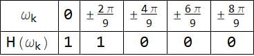
Hence, Equation 4 gives
$$h_{d}(n)= \frac{1}{9} \left( 1+2cos(\frac{2\pi}{9}n) \right)$$
Based on this equation, we obtain the corresponding time-domain representation as given by the following table:
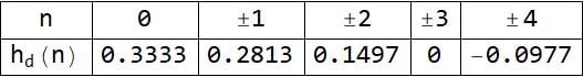
The frequency response of the designed filter is shown in Figure 6.
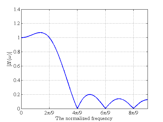
Figure 6. The frequency response of the filter designed in Example 1.
This figure shows that there are some ripples in the passband and stopband of the designed filter. These ripples make the obtained response deviate from that of the target ideal filter. However, note that, at $$\tfrac{2\pi}{9}k$$, $$k=0, 1, \dots, 8$$, the filter exhibits exactly the magnitude response that we were originally looking for (see Table 1). This can be explained by noting that the frequency sampling is based on the inverse DFT analysis. We applied the inverse DFT to the frequency domain samples of Table 1 and obtained the corresponding time-domain sequence, $$h_d(n)$$. Figure 6 is the frequency content of $$h_d(n)$$ and its equally-spaced samples at $$\tfrac{2\pi}{9}k$$, $$k=0, 1, \dots, 8$$ give the nine-point DFT of $$h_d(n)$$. Clearly, these samples should match those given by Table 1.
We can increase the number of the frequency domain samples to get a better approximation of the target filter and achieve a sharper transition. Obviously, this will require a filter of a higher order. The next example explains the design of a 25-tap filter for the lowpass filter of example 1.
Frequency Sampling Method Example 2
Use the frequency sampling method to design a 25-tap lowpass FIR filter with a cutoff frequency of $$0.25\pi$$ radians/sample.
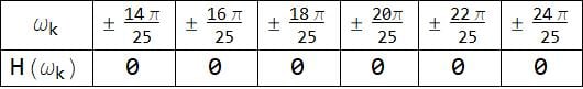
First, we find the value of the frequency response samples. Assuming an ideal response, the samples below $$0.25\pi$$ are equal to $$1$$ and the other samples are zero. Then, we obtain
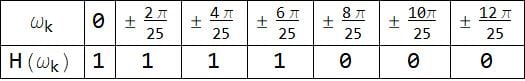
and
Hence, Equation 4 gives
$$h_{d}(n)= \frac{1}{25} \left( 1+2\left (cos(\frac{2\pi}{25}n)+cos(\frac{4\pi}{25}n)+cos(\frac{6\pi}{25}n) \right) \right)$$
Based on this equation, we obtain the corresponding time-domain representation as given by the following table:

and

The frequency response of the achieved 25-tap filter is shown in Figure 7.

Figure 7. The frequency response of the 25-tap filter with cutoff frequency of 0.25 radians/sample.
To reduce the passband ripples, we can employ a window function; however, this will increase the transition band and we may need to further increase the filter length to achieve a sharper response.
Summary
-
When $$H_d(\omega)$$ is given by a simple equation, we can easily calculate the integral of Equation 1. However, for an arbitrary $$H_d(\omega)$$, the frequency sampling method will be easier to apply.
-
For relatively small values of oversampling ratio (e.g., $$L \leq 8$$), we may need to compensate for the hold circuit distortion. To this end, we can design the interpolation filter to have a frequency response of $$\tfrac{1}{H_{DAC}}$$.
-
For $$N=2M+1$$ samples of $$H(\omega)$$, we can determine the filter coefficients of frequency sampling method using Equation 4.
Related Content