 Facebook
 Google
 GitHub
 Linkedin
FIR Filter Design by Windowing: Concepts and the Rectangular Window
In this article, we'll review the basic concepts in digital filter design. We'll also briefly discuss the advantages of FIR filters over IIR designs, e.g. stability and linear-phase response. Finally, we'll go over an introduction to designing FIR filters via the window method.
In this article, we'll review the basic concepts in digital filter design. We'll also briefly discuss the advantages of FIR filters over IIR designs, e.g. stability and the linear-phase response. Finally, we'll go over an introduction to designing FIR filters via the window method.
Why Do We Need Filters?
Filters are used in a wide variety of applications. Most of the time, the final goal of using a filter is to achieve a kind of frequency selectivity on the spectrum of the input signal.
As an example, suppose that a 50-Hz noise falls on top of the signal produced by a sensor. The noise component may be strong enough to limit the measurement precision. The output of the sensor is usually converted to a digital signal by an ADC to be processed by a DSP or a microcontroller. Therefore, we can use a digital filter after the ADC to eliminate the noise component. In this particular example, a notch filter centered at 50 Hz can be utilized to suppress the noise.
At this point, it is worth reviewing the frequency response of a practical filter. Figure (1) shows an example of a practical lowpass filter. In this example, frequency components in the passband, from DC to $$\omega_{ p}$$, will pass through the filter almost with no attenuation. The components in the stopband, above $$\omega_{s}$$, will experience significant attenuation. Note that the frequency response of a practical filter cannot be absolutely flat in the passband or in the stopband. As shown in Figure (1), some ripples will be unavoidable and the transition band, $$\omega_{p}< \omega< \omega_{s}$$ , cannot be infinitely sharp in practice.
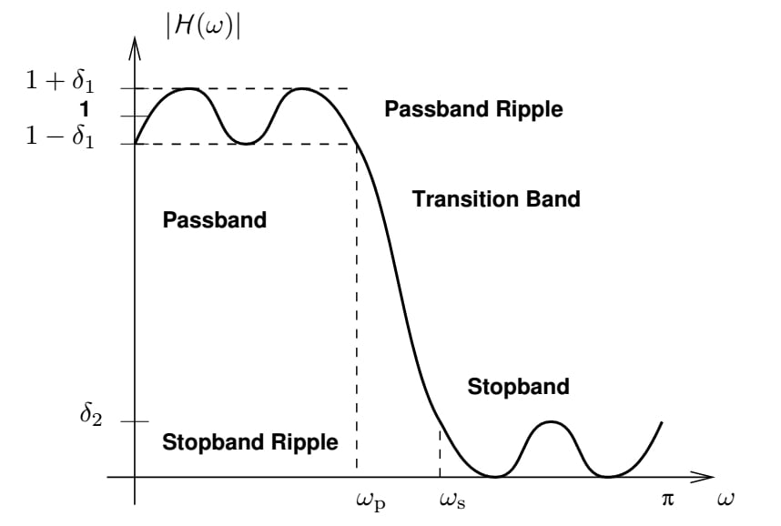
Figure (1) Frequency response of a practical lowpass filter. Image courtesy of the University of Michigan (PDF).
General Considerations
Digital filter design involves four steps:
1) Determining specifications
First, we need to determine what specifications are required. This step completely depends on the application. In the example of 50-Hz noise on the output of the sensor, we need to know how strong the noise component is relative to the desired signal and how much we need to suppress the noise. This information is necessary to find the filter with minimum order for this application.
2) Finding a transfer function
With design specifications known, we need to find a transfer function which will provide the required filtering. The rational transfer function of a digital filter is as in Equation (1).
$$H(z)=\frac{\sum_{k=0}^{M-1}b_{k}z^{-k}}{\sum_{k=0}^{N-1}a_{k}z^{-k}}$$
Equation (1)
This step calculates the coefficients, $$a_{k}$$ and $$b_{k}$$, in Equation (1).
3) Choosing a realization structure
Now that $$H(z)$$ is known, we should choose the realization structure. In other words, there are many systems which can give the obtained transfer function and we must choose the appropriate one. For example, any of the direct form I, II, cascade, parallel, transposed, or lattice forms can be used to realize a particular transfer function. The main difference between the aforementioned realization structures is their sensitivity to using a finite length of bits. Note that in the final digital system, we will use a finite length of bits to represent a signal or a filter coefficient. Some realizations, such as direct forms, are very sensitive to quantization of the coefficients. However, cascade and parallel structures show smaller sensitivity and are preferred.
4) Implementing the filter
After deciding on what realization structure to use, we should implement the filter. You have a couple of options for this step: a software implementation (such as a MATLAB or C code) or a hardware implementation (such as a DSP, a microcontroller, or an ASIC).
This article focuses on the second step in designing an FIR filter.
FIR Filters
An FIR filter is a special case of Equation (1), where $$a_{0}=1$$ and $$a_{k}=0$$ for $$k=1,...,N-1$$, hence we obtain:
$$H(z)=\sum_{k=0}^{M-1}b_{k}z^{-k}$$
Equation (2)
The direct form realization of Equation (2) for M=3 is shown in Figure (2). As shown in this figure, a digital filter can be implemented using only three elements:
- Addition
- Multiplication by a constant (necessary for the implementation of the coefficients)
- Delay blocks
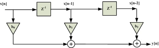
Figure (2) Direct form of an FIR filter of order 2
There are three coefficients and two delay cells in Figure (2). Note that this filter is of order 2, the number of delay cells, not 3, the number of coefficients.
An FIR filter has two important advantages over an IIR design:
Firstly, as shown in Figure (2), there is no feedback loop in the structure of an FIR filter. Due to not having a feedback loop, an FIR filter is inherently stable. Meanwhile, for an IIR filter, we need to check the stability.
Secondly, an FIR filter can provide a linear-phase response. As a matter of fact, a linear-phase response is the main advantage of an FIR filter over an IIR design—otherwise, for the same filtering specifications, an IIR filter will lead to a lower order.
In order to have a linear-phase FIR filter, we must provide symmetry in the time domain, i.e. $$b[n]=\pm b[M-1-n]$$. In the example shown in Figure (2), assume that $$b_{0}=b_{2}$$, hence Equation (2) gives
$$H(z)=b_{0}+b_{1} e^{-j\omega}+b_{0} e^{-j2\omega}=e^{-j\omega} (b_{1}+2b_{0} cos(\omega))$$
Equation (3)
Since $$b_{k}$$ is real, phase of $$H(z)$$ will be
$$\measuredangle H(z)=\left\{\begin{matrix}-\omega_{p}
& b_{1}+2b_{0}cos(\omega)>0\\ -\omega_{p}+\pi
& b_{1}+2b_{0}cos(\omega)<0
\end{matrix}\right.$$
Equation (4)
Therefore, the phase response will be linear. Although this example shows a linear-phase response in the case of a three-tap filter, it can be shown that for an arbitrary value of $$M$$, time-domain symmetry leads to a linear-phase response. This is an important property which helps us to examine the linear-phase response of an FIR filter just by considering the values of $$b_{k}$$ without any calculation.
The reader may wonder why a linear-phase frequency response is important. To gain insight, consider the continuous-time case. Assume that the frequency response of a system is
$$H(s)=\alpha e^{-j \beta \omega}$$
Equation (5)
where $$\alpha$$ and $$\beta$$ are real constants. The phase response of this system is linear, i.e. $$\measuredangle H(s)=-\beta\omega$$.
If we apply $$x(t)=Acos(\omega_{1}t)$$ to this system, the output will be $$y(t)=\alpha A cos(\omega_{1} t - \beta \omega_{1})=\alpha x(t-\beta)$$. Therefore, the linear-phase response corresponds to a constant delay. A system with a nonlinear-phase response will distort the input, even if $$\left | H(s) \right |$$ is constant. In such a system, different frequency components of the input will experience different time delays as they pass through the system. For a digital system with a phase response of $$\measuredangle H(z)=-k\omega$$ where $$k$$ is an integer, we can also prove that the linear phase is equal to a constant delay.
Introduction to FIR Filter Design by Windowing
We will explain the window method by using an example. Suppose that we want to design a lowpass filter with a cutoff frequency of $$\omega_{c}$$, i.e. the desired frequency response will be:
$$H_{d} (\omega)=\left\{\begin{matrix}
1 & \left | \omega \right |<\omega_{c}\\0
& else
\end{matrix}\right.$$
Equation (6)
To find the equivalent time-domain representation, we calculate the inverse discrete-time Fourier transform:
$$h_{d} [n]=\frac{1}{2\pi} \int_{-\pi}^{+\pi}H_{d}(\omega)e^{j\omega n}d\omega$$
Equation (7)
Substituting Equation (6) into Equation (7), we obtain:
$$h_{d} [n]=\frac{1}{2\pi} \int_{-\omega_{c}}^{+\omega_{c}}e^{j\omega n}d\omega=\frac{sin(n\omega_{c})}{n\pi}$$
Equation (8)
Equation (8) for $$\omega_{c}=\frac{\pi}{4}$$ is shown in Figure (3):
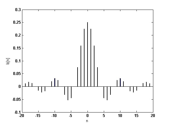
Figure (3) Impulse response of an ideal lowpass filter with $$\omega_{c}=\frac {\pi} {4}$$
Figure (3) shows that $$h_{d}[n]$$ needs an infinite number of input samples to perform filtering and that the system is not a causal system.
The obvious solution will be to truncate the impulse response and use, for example, only 21 samples of the input and assume other coefficients to be zero. Intuition suggests that, as the number of samples increases, the truncated impulse response will be closer to the ideal impulse response in Figure (3) and therefore the frequency response of the achieved filter will be closer to Equation (6).
On the other hand, as we increase the number of samples, more hardware will be required. If we choose to use only 21 taps of the ideal response, there will be three options which are shown in Figures (4) to (6).
The first option is shown in Figure (4). This impulse response corresponds to a non-causal system and cannot be used.
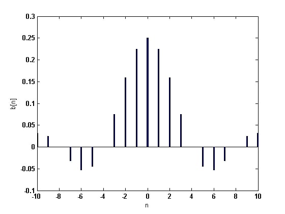
Figure (4) Truncated impulse response: linear-phase, but non-causal
The next option is shown in Figure (5) which, despite being causal, does not have a linear-phase response (the most important property of an FIR system).
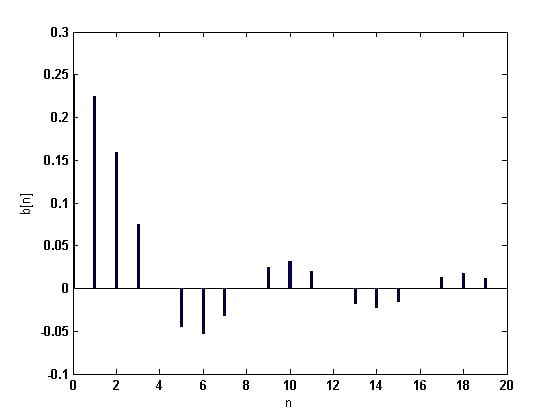
Figure (5) Truncated impulse response: causal, but nonlinear-phase
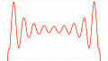
The last option is shown in Figure (6). This system is both causal and linear phase. The only drawback to this system is its delay which is $$\frac{M-1}{2}$$ samples. In other words, in response to an impulse at $$n=0$$, the system will not react until almost $$n=\frac{M-1}{2}$$. This delay may cause problems in some applications.
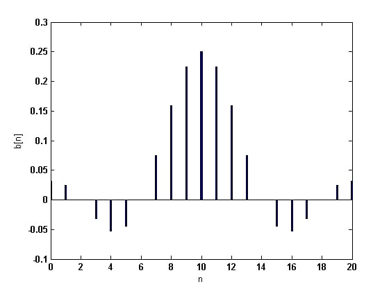
Figure (6) Truncated impulse response: causal and linear phase
Truncation of the impulse response is equivalent to multiplying $$h_{d}[n]$$ (or its shifted version) by a rectangular window, $$w[n]$$ which is equal to one for $$n=0,...,M-1$$ and zero otherwise. Therefore, considering the applied shift, we obtain the impulse response of the designed filter:
$$h[n]=h_{d} [n-\frac{M-1}{2}]w[n]$$
Equation (9)
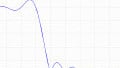
Clearly the spectrum of the rectangular window will cause the filter response to deviate from the ideal response in Equation (6). Figure (7) compares the response of the designed filter with that of the ideal one.
This figure shows that, unlike the ideal filter, the designed filter has a smoother transition from the passband to the stopband. Moreover, there are some ripples in both the passband and stopband of $$H(\omega)$$ . How can we make the transition band sharper? How can we make the ripples smaller? What other options are there to be used instead of a rectangular window?
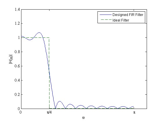
Figure (7) Frequency response of the filter designed by a rectangular window
Summary
- To design a digital filter, we need to find the coefficients, $$a_{k}$$ and $$b_{k}$$, in Equation (1).
- An FIR filter is a special case of Equation (1), where $$a_{0}=1$$ and $$a_{k}=0$$ for $$k=1,...,N-1$$.
- Stability and linear-phase response are the two most important advantages of an FIR filter over an IIR filter.
- A linear-phase frequency response corresponds to a constant delay.
- Truncation of the impulse response is equivalent to multiplying $$h_{d}[n]$$ by a rectangular window, $$w[n]$$, which is equal to one for $$n=0,...,M-1$$ and zero otherwise.
- A wider transition band and ripples in the passband and stopband are the most important differences between the ideal filters and those designed by window method.


I took an Intro to DSP course in college and loved it. Then took a DSP and Bioengineering course where I had to design a IIR filter. I failed. I couldn’t get it to converge. I was wondering if you had any resources to help me understand the design process of a IIR filter. Just a place to get started.