Facebook
 Google
 GitHub
 Linkedin
From Filter Specs to Window Parameters in FIR Filter Design
Learn how to use filter specs to help choose the best window parameters for your FIR filter design.
Learn how to use filter specs to help choose the best window parameters for your FIR filter design.
The previous article in this series discussed that a tapered window, such as a Bartlett, can give better PSL than a rectangular window which has abrupt variation in the time domain.
In this article, first, we will review other popular windows. Then, we will clarify the design procedure by calculating the cutoff of the ideal filter, window type, and window length from given filter specs, namely, $$\omega_{p}$$, $$\omega_{s}$$ and $$\delta$$.
In other words, a specific application gives us $$\omega_{p}$$, $$\omega_{s}$$, and $$\delta$$, and now we need to find the required ideal filter response, window type, and window length to design an FIR filter. The relation between these parameters is the subject of this article.
Other Popular Window Functions
Fortunately, the Bartlett and the rectangular windows are not the only options in FIR filter design and many other windows have been developed.
Table I shows some of the most popular windows along with their important properties. In Table I, Bartlett, Hann, and Hamming have equal approximate main lobe width, but we can observe the general trade-off between the PSL and the main lobe width. The rectangular window has the smallest main lobe width and the largest PSL, whereas the Blackman has the widest main lobe and the smallest PSL.
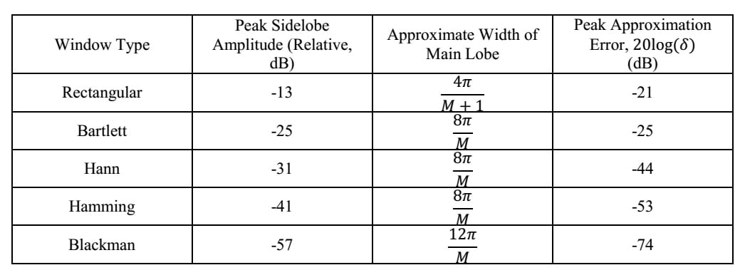
Table I Popular windows and their properties.
The Fourier transform of three windows, Bartlett, Hann, and Hamming with $$M=21$$, are plotted in Figure (1). The mentioned trade-off is observed in these three windows, too. As the PSL reduces, the main lobe width increases.
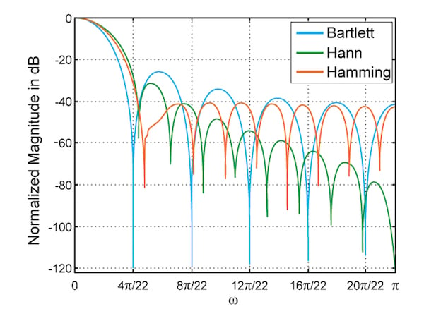
Figure (1) Bartlett, Hann, and Hamming of length $$M=21$$.
In addition to PSL and approximate main lobe width, Table I gives, for each window, the peak approximation error, which is the deviation from the ideal response (denoted by $$\delta$$) expressed in dB. This is an important parameter which allows us to choose an appropriate window based on the requirements of an application. Peak approximation error determines how much deviation from the ideal response we expect for each of the window types. This is illustrated in Figure (2).
As will be discussed in the following section, the deviations from the ideal response in the pass-band and stop-band are approximately equal when using the window method to design FIR filters, i.e., $$\delta_{1}=\delta_{2}=\delta$$. Therefore, we can select the suitable window based on how much ripple is allowed in the pass-band or how much attenuation is needed in the stop-band.
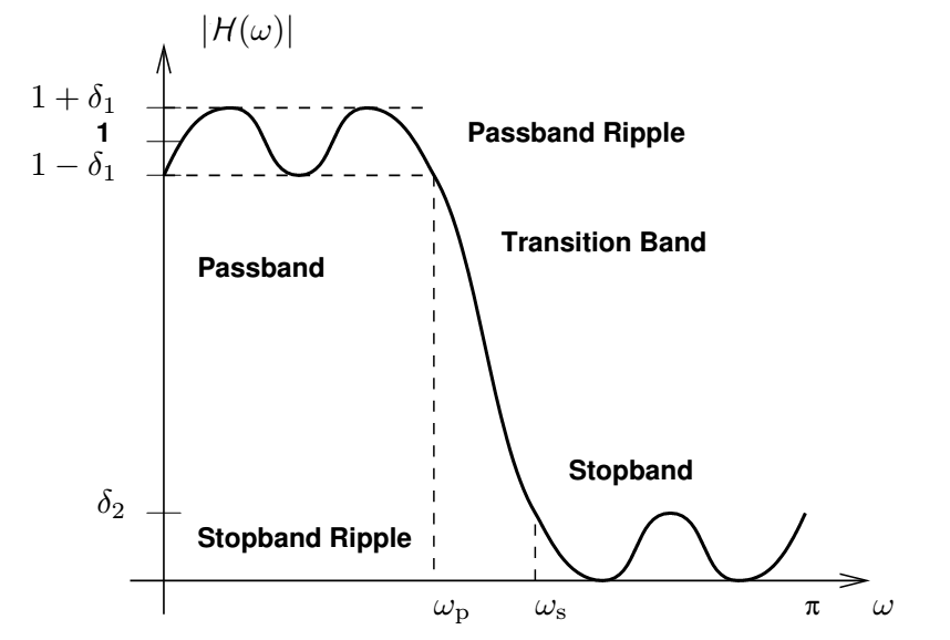
Figure (2) Deviations from the ideal response in the pass-band, $$\delta_{1}$$, and in the stop-band, $$\delta_{2}$$. Image courtesy of the University of Michigan (PDF).
Important Properties of the Window Method
In this section, some of the most important properties of the window method, which are necessary for design procedure, will be discussed. We need to find the cutoff of the ideal filter, window type, and length based on given filter specs, namely, $$\omega_{p}$$, $$\omega_{s}$$, and $$\delta$$. In other words, a specific application gives us $$\omega_{p}$$, $$\omega_{s}$$, and $$\delta$$, and now we need to find the required ideal filter response, window type, and window length to design an FIR filter. The relation between these parameters is the subject of this section.
Please note that we are not trying to give strict and thorough proofs. Instead, our goal is to provide some insight into these properties so that you do not need to memorize them.
1- Ideal Cutoff Frequency, $$\omega_{p}$$ and $$\omega_{s}$$
When using the window method to design an FIR filter, we start from filter specs $$\omega_{p}$$ and $$\omega_{s}$$. Having $$\omega_{p}$$ and $$\omega_{s}$$, we should find a suitable ideal filter with cutoff frequency $$\omega_{c}$$, then find the FIR filter related to this ideal filter.
The question is: What is the relation between $$\omega_{p}$$, $$\omega_{s}$$ and $$\omega_{c}$$?
To answer this question, consider Figure (3). This figure shows the slide-and-integrate process, discussed in a previous article of this series, to calculate the convolution of the window and the ideal filter. The ideal desired frequency response, the designed filter, and the shifted window spectrum are shown in this figure. Note that the Fourier transform of the window is approximated with only the main lobe and the first sidelobes (the amplitude of the other sidelobes is assumed to be zero). The window is shifted so that its peak is exactly on the abrupt cutoff of the ideal filter.
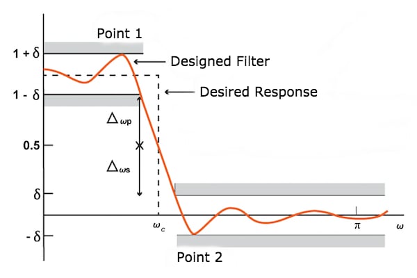
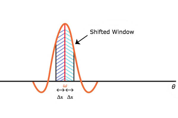
Figure (3) The Fourier transform of the window is symmetric around its peak and hence $$\omega_{c}=\frac{\omega_{p}+\omega_{s}}{2}$$.
First, assume that we shift the window from its current position by $$\Delta x$$ to the right. The part of the window marked by the red dashed lines will go out of the passband of the ideal filter. Hence, the convolution value will decrease by, let’s say $$\Delta_{1}$$.
Now, assume that we shift the window from its position in Figure (3) by $$\Delta x$$ to the left. The part of the window which is marked by the blue dashed lines will go inside the passband of the ideal response. How much will the convolution increase by?
Since the Fourier transform of the window is symmetrical around its peak, the convolution will increase by $$\Delta_{1}$$. Note that this reasoning may be invalid if we do not assume that the main lobe with is much smaller than the passband of the ideal filter (Why do you think this might be the case? See if you can come up with the answer on your own.)
With this symmetrical behavior in mind, consider $$\omega_{p}$$ where the magnitude of frequency response is $$1-\delta$$ and where $$\Delta_{\omega p}$$, as shown in Figure (3), will be $$1-\delta-0.5$$ in this case.
At $$\omega_{s}$$, the magnitude of frequency response will be $$\delta$$ and $$\Delta_{\omega s}$$, as shown in Figure (3), will be $$0.5-\delta$$. Since $$\Delta_{\omega p}=\Delta_{\omega s}$$, we can conclude that frequency shifts corresponding to these two cases are equal.
In other words, $$\omega_{c}=\frac{\omega_{p}+\omega_{s}}{2}$$. Notice that, as shown in the figure, the magnitude of the designed filter is approximately 0.5 at $$\omega=\omega_{c}$$. This is quite obvious in the special case of ignoring all the sidelobes and keeping only the main lobe.
2- Peak Approximation Error in Pass-Band and Stop-Band
The peak approximation error in the pass-band is equal to the peak approximation error in the stop-band. To get a feeling for this, consider Figure (4) which is taken from a previous article in this series.
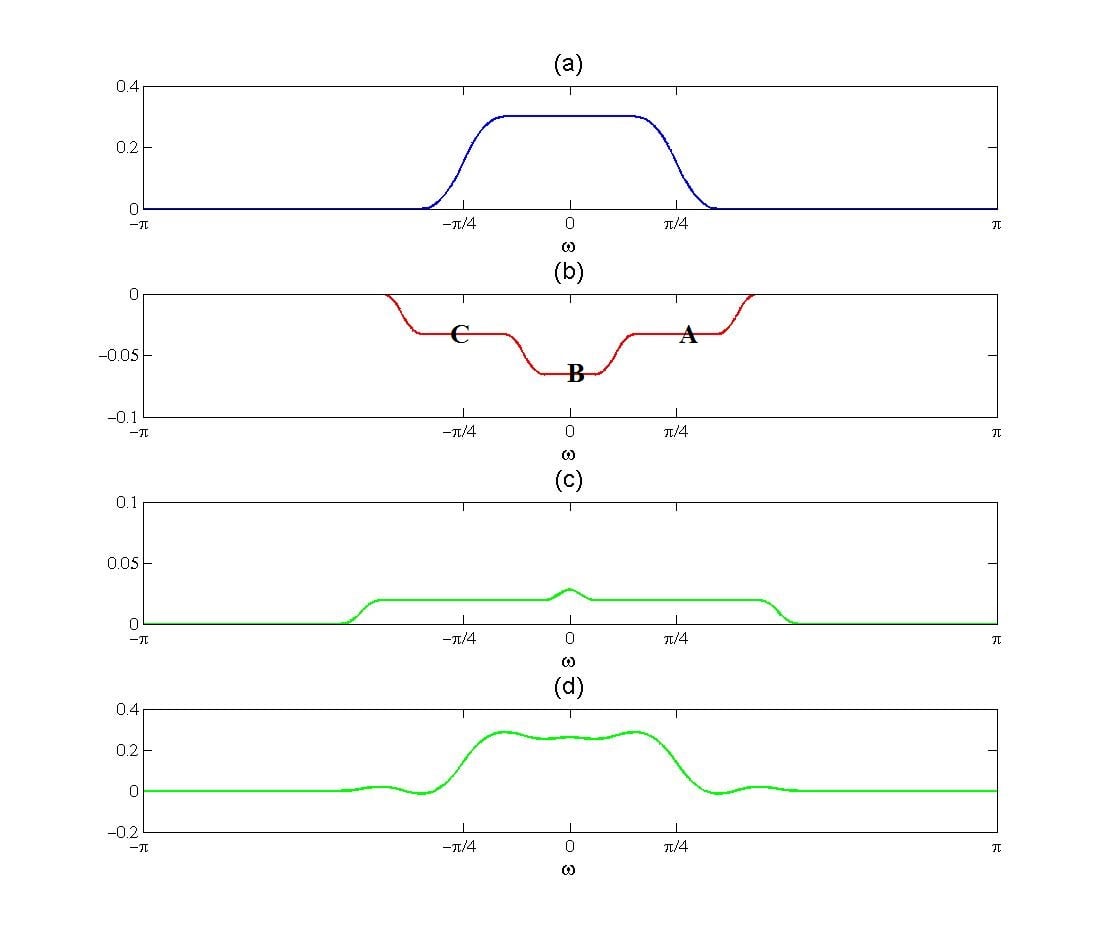
Figure (4) Convolution of $$H_{d}(\omega)$$ with (4a) $$T_{1}$$ (4b) $$T_{2}$$ (4c) $$T_{3}$$ and (4d) $$T_{1}+T_{2}+T_{3}$$
This figure shows the convolution of the ideal response with triangular approximations of the main lobe, $$T_{1}$$, the first sidelobe, $$T_{2}$$, and second sidelobe, $$T_{3}$$.
Peak approximation error is directly related to the PSL of the window. In fact, other side lobes are much smaller than the first sidelobe and have a negligible effect on the peak approximation error.
If we assume that the main lobe width of the window is much smaller than the cutoff frequency, $$\omega_{c}$$, of the ideal filter, $$H_{d}(\omega)$$, the convolution of $$H_{d}(\omega)$$ with $$T_{1}$$ and $$T_{2}$$ will be similar to Figure (4a) and (4b), respectively.
We know that the convolution of $$H_{d}(\omega)$$ with $$T_{2}$$ determines the ripples in the frequency response of the designed filter. In Figure (4b), $$H_{d}(\omega)*T_{2}$$ has a variation of one step, A and C, at the stop-band. Besides, $$H_{d}(\omega)*T_{2}$$ has a variation of only one step, B, in the pass-band.
Since the variation of $$H_{d}(\omega)*T_{2}$$ is the same in both the pass-band and the stop-band, we expect the peak approximation error to be the same in both the stop-band and pass-band.
3- Transition Band and the Main Lobe Width
Having $$\omega_{p}$$ and $$\omega_{c}$$, we need to determine the main lobe width of the required window. To this end, we examine Figure (3) one more time. As shown in Figure (3), we only consider the first sidelobe.
In this figure, if we shift the window to the left so that the main lobe is completely inside the passband of the ideal filter response, we will get the maximum of the convolution, point1 in the figure.
On the other hand, if we shift the window to the right so that the main lobe is right out of the ideal response, point2 will be achieved.
Therefore, the distance between point1 and point2 is almost equal to the main lobe width. As a result, the transition band, $$\omega_{s}-\omega_{p}$$, will be smaller than the main lobe width. However, we can use the transition band as an estimate of the required main lobe width.
Summary
- When using the window method to design an FIR filter, we start from filter specs $$\omega_{p}$$, $$\omega_{s}$$ and $$\delta$$.
- Having $$\delta$$, we can choose the appropriate window type from Table I.
- We can use the transition band, $$\omega_{s}-\omega_{p}$$, as an estimate of the required main lobe width and therefore find the window length from Table I.
- Having $$\omega_{p}$$ and $$\omega_{s}$$, we can find the suitable ideal filter with cutoff frequency of $$\omega_{c}=\frac{\omega_{p}+\omega_{s}}{2}$$ and then find the FIR filter corresponding to this ideal filter.
Related Content