Design Examples of FIR Filters Using the Window Method

This article gives several design examples of FIR filters using the window technique.

Based on the previous articles in this series, especially the last one, we will discuss a step-by-step design procedure.

Please note that, in this article, we will use "stop-band attenuation" and "the minimum stop-band attenuation" interchangeably.

Example 1:

Design a low-pass filter with $$\omega_{p}=0.4\pi$$ and $$\omega_{s}=0.6\pi$$ which exhibits a minimum attenuation greater than $$50dB$$ in the stop-band.

 

1) Choose the Window Type

An ideal low-pass filter has infinite attenuation in the stop-band. When we approximate an ideal filter with a practical filter using the window method, we accept some approximation error. The peak approximation error depends on the window type and is known for each window as reported in Table I.

Table I: Popular window functions and their properties

 

Considering the fact that the stop-band attenuation of an ideal filter is infinite, we find that the peak approximation error of the utilized window determines the stop-band attenuation of the designed filter.

Since we need attenuation greater than $$50dB$$ in the stop-band, we may use either the Hamming or the Blackman from Table I.

The Blackman window will lead to an overdesigned filter. This is due to the fact that, for a given window length, $$M$$, the Blackman gives a wider main lobe which is not desired. Hence, in this example, use of the Blackman will force us to use a larger $$M$$ compared to utilizing the Hamming window.

Among the five windows in Table I, Hamming is the appropriate window for this example.

2) Approximate the Window Length

As discussed in the previous article, we can find a rough estimation of the window length by equating the transition band of the filter with the main lobe width of the window.

In this example, the transition band is $$\omega_{s}-\omega_{p}=0.2\pi$$. Since the main lobe width of the Hamming window is approximately $$\frac{8\pi}{M}$$, we find $$M=40$$. This means that the designed filter will be of length $$41$$.

So far we have determined the window type and its length. Using the equation describing a Hamming window, we find the window as

 

$$w[n]=\left\{\begin{matrix} 0.54-0.46cos(\frac{2n\pi}{M}) & 0 \leq n \leq M \\ 0 & otherwise \end{matrix}\right \}$$

Equation (1)

 

where $$M=40$$.

3) Find the Appropriate Ideal Filter

Based on the previous article in this series, we know that the cut-off frequency of the ideal filter is $$\omega_{c}=\frac{\omega_{p}+\omega{s}}{2}$$. Hence, in this example, we need to find the impulse response of an ideal low-pass filter with $$\omega_{c}=0.5\pi$$. Equation (8) of a previous article in this series calculated the impulse response of a low-pass filter with cut-off frequency of $$\omega_{c}$$ as

 

$$h_{d,lowpass}[n]=\frac{\omega_{c}}{\pi}sinc(\frac{\omega_{c}n}{\pi})$$

Equation (2)

 

Hence, in this example, we obtain

 

$$h_{d,lowpass}[n]=0.5sinc(\frac{n}{2})$$

4) Apply a time shift of $$\frac{M}{2}$$ and multiply $$h_{d,lowpass}[n]$$ by $$w[n]$$ 

To have a causal linear-phase response, we need to apply a time shift equal to $$\frac{M}{2}$$ in the ideal impulse response and multiply the result by $$w[n]$$. Therefore, we find

 

$$h[n]=\begin{matrix} [0.54-0.46cos(\frac{2n\pi}{M})][0.5sinc(\frac{n-20}{2})] & 0 \leq n \leq M \end{matrix}$$

 

where $$h[n]$$ denotes the impulse response of the designed FIR filter.

The frequency response of the designed low-pass filter is shown in Figure (1):

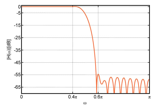
Figure (1) Magnitude response of the low-pass filter in Example 1

 

The simulated frequency response exhibits an attenuation of $$55dB$$ in the stop-band which is very close to the rejection predicted by the peak approximation error of the Hamming window. As shown in Figure (1) and (2), $$\omega_{p}$$ and $$\omega_{s}$$ are slightly different from the design specifications, however, the differences are negligible.

As discussed in the previous article in this series, the window method leads to the same ripple in the pass-band and stop-band. However, since Figure (1) uses a logarithmic scale for $$|H(\omega)|$$, the ripples in the stop-band seem to be larger. This is due to the fact that variation of a logarithmic function is much larger when its argument is close to zero.   

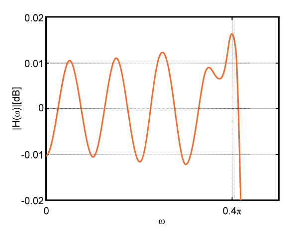
Figure (2) Zoomed-in version of the pass-band of the designed low-pass filter

 

Note that we always need software verification of any design, however, hand calculations give us a better understanding of the problem and enable us to have a rough approximation of the system. In this example, simple hand calculations enable us to roughly approximate the value of $$M$$.

Example 2:

Design a high-pass filter with $$f_{s}=200Hz$$ and $$f_{p}=300Hz$$ which exhibits attenuation greater than $$40dB$$ in the stop-band. We need the pass-band ripple to be less than $$0.2dB$$. Assume that the sampling frequency, $$f_{samp}$$, is $$1200Hz$$.

1) Window Type

Figure (3) shows the ripples in the pass-band and stop-band of a practical filter.

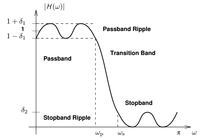
Figure (3) Pass-band and stop-band ripples of a practical filter. Image courtesy of the University of Michigan (PDF).

 

Although this figure shows a low-pass filter, the relations for the ripples are valid for other filter types. Considering Figure (3), we can find the pass-band ripple as $$20log(1+\delta_{1})-20log(1)=20log(1+\delta_{1})$$. In this example, $$20log(1+\delta_{1})=0.2dB$$, hence $$\delta_{1}=0.023$$.

The stop-band attenuation is $$-20log(\delta_{2})=40dB$$ which gives $$\delta_{2}=0.01$$. We discussed that, with the window method, the peak approximation error is the same in the pass-band and the stop-band. As a result, we need to choose the peak approximation error as the minimum of $$\delta_{1}$$ and $$\delta_{2}$$. Therefore, $$\delta=0.01$$ and the peak approximation error is $$-40dB$$.

From the window functions of Table I, we can use Hann, Hamming, or Blackman among which Hann will lead to the smallest window length.

2) Window Length

We can find the approximate window length by equating the main lobe width with the transition band of the desired filter. Note that since this example discusses a high-pass filter, $$\omega_{p}$$ is greater than $$\omega_{s}$$. Moreover, this example gives the pass-band and stop-band frequencies in Hz.

To find the angular frequencies, we need to normalize $$f_{s}$$ and $$f_{p}$$ with half the sampling frequency and multiply the result by $$\pi$$. Therefore, $$\omega_{p}=2\pi \frac{f_{p}}{f_{samp}}=0.5\pi$$ and $$\omega_{s}=0.33\pi$$.

Equating the transition band, $$0.17\pi$$, with the main lobe width of the Hann window, we obtain $$M=47$$. An odd M will lead to a type II filter which is not suitable for high-pass and band-stop filters. As a result, we need to increase the filter length by one, i.e. $$M=48$$.

Using the equation describing a Hann window, we find the window as

 

$$w[n]=\left\{\begin{matrix} 0.5-0.5cos(\frac{2n\pi}{M}) & 0 \leq n \leq M \\ 0 & otherwise \end{matrix}\right \}$$

Equation (3)

 

where $$M=48$$.

3) Find the Appropriate Ideal Filter

The cut-off frequency of the high-pass filter will be $$\omega_{c}=\frac{\omega_{p}+\omega_{s}}{2}=\frac{0.5\pi+0.33\pi}{2}=0.415\pi$$. To find the impulse response of a high-pass filter, note that a high-pass filter with cut-off frequency of $$\omega_{c}$$ is the subtraction of a low-pass filter with cut-off of $$\omega_{c}$$ from a low-pass with cut-off of $$\pi$$.

Using the impulse response of a low-pass filter given by Equation (2), we can find the impulse response of a high-pass filter with cut-off of $$\omega_{c}$$ as

 

$$h_{d,highpass}[n]=sinc(n)-\frac{\omega_{c}}{\pi}sinc(\frac{\omega_{c}n}{\pi})$$

Equation (4)

 

In this example, the ideal impulse response will be

 

$$h_{d,highpass}[n]=sinc(n)-0.415sinc(0.415n)$$

4) Apply the time shift and multiply $$h_{d,highpass}[n]$$ by $$w[n]$$

The impulse response of the designed filter will be

 

$$h[n]=\begin{matrix} [0.5-0.5cos(\frac{2n\pi}{48})][sinc(n)-0.415sinc(0.415n)] & 0 \leq n \leq M \end{matrix}$$

 

The frequency response of the designed high-pass filter is shown in Figure (4).

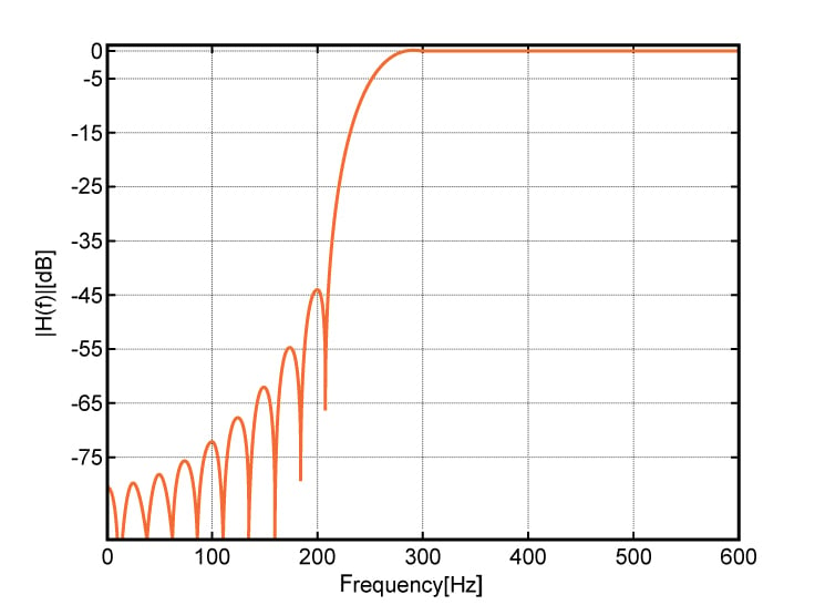
Figure (4) Magnitude response of the high-pass filter in Example 2

 

The simulated frequency response exhibits an attenuation of $$45dB$$ in the stop-band which is very close to the rejection predicted by the peak approximation error of the Hann window.

As shown in Figure (4) and (5), $$f_{p}$$ and $$f_{s}$$ are slightly different from the design specifications, however the differences are negligible. By tweaking $$M$$, $$f_{p}$$ or $$f_{s}$$, we can find filters that are closer to the design specifications.

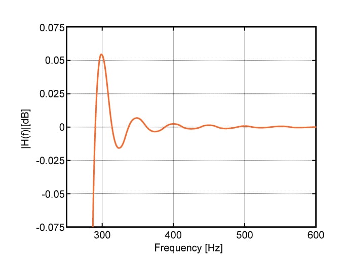
Figure (5) Zoomed-in version of the pass-band of the designed high-pass filter.

Example 3:

Design a band-pass filter with center frequency and two-sided pass-band of $$f_{center}=500Hz$$ and $$300Hz$$, respectively. Both the low and high transition bands of this filter are $$100Hz$$. The stop-band rejection needs to be greater than $$60dB$$ and the pass-band ripple is expected to be less than $$0.1dB$$. Assume that the sampling frequency, $$f_{samp}$$, is $$2000Hz$$.

1) Window Type

Assume that, similar to the low-pass example in Figure (3), $$\delta_{1}$$ and $$\delta_{2}$$ denote the deviation from ideal response in the pass-band and stop-band, respectively. Therefore, $$20log(1+\delta_{1})=0.1$$ and $$20log(\delta_{2})=-60$$. We need to choose the peak approximation error of the design based on the minimum of $$\delta_{1}$$ and $$\delta_{2}$$. Hence we obtain $$\delta=min\{\delta_{1}, \delta_{2}\}=0.001$$. The Blackman is the only window in Table I which can provide a peak approximation error smaller than $$-60dB$$.

2) Window Length

The angular transition band is found as $$\Delta\omega=2\pi\frac{\Delta f}{f_{samp}}=2\pi\frac{100}{2000}=0.1\pi$$. Equating the transition band, $$0.1\pi$$, with the main lobe width of the Blackman window, we obtain $$M=120$$.

Using the equation describing the Blackman window, we find the window as

 

$$w[n]=\left\{\begin{matrix} 0.42-0.5cos(\frac{2n\pi}{M})+0.08cos(\frac{4n\pi}{M}) & 0 \leq n \leq M \\ 0 & otherwise \end{matrix}\right \}$$

Equation (5)

 

where $$M=120$$.

3) Find the Appropriate Ideal Filter

Consider a band-pass filter with the low cut-off and high cut-off of $$\omega_{c,l}$$ and $$\omega_{c,u}$$, respectively. The impulse response of this band-pass filter can be found by subtracting the response of two low-pass filters with cut-off frequencies of $$\omega_{c,u}$$ and $$\omega_{c,l}$$. Utilizing Equation (2), we can arrive at the impulse response of the assumed band-pass filter as

 

$$h_{d,bandpass}[n]=\frac{\omega_{c,u}}{\pi}sinc(\frac{\omega_{c,u}n}{\pi})-\frac{\omega_{c,l}}{\pi}sinc(\frac{\omega_{c,l}n}{\pi})$$

Equation (6)

 

In this example, the ideal impulse response will be

 

$$h_{d,bandpass}[n]=0.7sinc(0.7n)-0.3sinc(0.3n)$$

4) Apply the time shift and multiply $$h_{d,bandpass}[n]$$ by $$w[n]$$ 

The impulse response of the designed filter will be

 

$$h[n]=\begin{matrix} [0.42-0.5cos(\frac{n\pi}{60})+0.08cos(\frac{n\pi}{30})][0.7sinc(0.7(n-60))-0.3sinc(0.3(n-60))] & 0 \leq n \leq 120 \end{matrix}$$

 

The frequency response of the designed band-pass filter is shown in Figure (6).

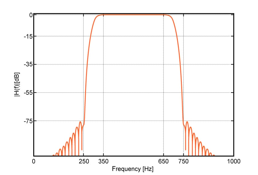
Figure (6) Magnitude response of the band-pass filter in Example 3

 

The simulated frequency response exhibits an attenuation of $$75dB$$ in the stop-band which is very close to the rejection predicted by the peak approximation error of the Blackman window. As shown in Figure (6) and (7), $$f_{p}$$ and $$f_{s}$$ are very close to the design specifications.

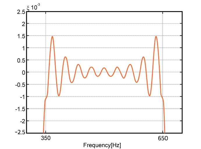
Figure (7) Zoomed-in version of the pass-band of the designed band-pass filter

I hope you now have more practical knowledge of how to use the window method to design FIR Filters.

 

• ← Previous Article
• Next Article →