Structures for Implementing Finite Impulse Response Filters

This article will review some basic structures to implement Finite Impulse Response (FIR) filters.

When designing a filter, we start from a set of specifications which are generally determined by a particular application. For example, we may need to suppress the 50-Hz noise which appears at the output of a sensor and makes our measurements inaccurate. Based on the frequency and strength of the noise component, we can determine the filter specifications such as the passband and stopband edge, the transition bandwidth, the ultimate out-of-band rejection, etc. Now, we can find the system function, $$H(z)$$, which satisfies these requirements.

For a FIR design, we have a couple of options such as the windowing method, the frequency sampling method, and more. Then, we need to choose a realization structure for the obtained system function. In other words, there are several structures which exhibit the same system function $$H(z)$$. One consideration for choosing the appropriate structure is the sensitivity to coefficient quantization. Since a digital filter uses a finite number of bits to represent signals and coefficients, we need structures which can somehow retain the target filter specifications even after quantizing the coefficients. In addition, sometimes we observe that a particular structure can dramatically reduce the computational complexity of the system.

The Direct-Form Structure

The direct-form structure is directly obtained from the difference equation. Assume that the difference equation of the FIR filter is given by

$$y(n)=\sum_{k=0}^{M-1}b_{k}x(n-k)$$

Equation 1

Based on the above equation, we need the current input sample and $$M-1$$ previous samples of the input to produce an output point. For $$M=5$$, we can simply obtain the following diagram from Equation 1.

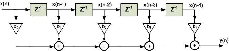
Figure 1. Direct-form structure for a fourth-order FIR filter.

Using the direct-form realization of Figure 1, we need $$M$$ multipliers for an $$(M-1)$$th-order FIR filter. However, usually, we can almost halve the number of multipliers. This can be achieved by noting that we are mainly interested in linear-phase FIR filters. In fact, the main advantage of a FIR filter over an infinite impulse response (IIR) design is its linear-phase response, otherwise, for a given set of specifications, an IIR design can offer a filter of lower order and reduce the computational complexity. On the other hand, for a linear-phase FIR filter, we observe the following symmetry in the coefficients of the difference equation

$$b_{k}=\pm b_{M-1-k}$$

For $$M=5$$, Equation 1 gives

$$y(n)=b_{0}x(n)+b_{1}x(n-1)+b_{2}x(n-2)+b_{3}x(n-3)+b_{4}x(n-4)$$

Assuming $$b_{k}=b_{M-1-k}$$, we obtain

$$y(n)=b_{0}\left( x(n) + x(n-4) \right)+b_{1}\left( x(n-1)+x(n-3) \right)+b_{2}x(n-2)$$

The structure obtained from the above equation is shown in Figure 2. While Figure 1 requires five multipliers, employing the symmetry of a linear-phase FIR filter, we can implement the filter using only three multipliers. This example shows that for an odd $$M$$, the symmetry property reduces the number of multipliers of an $$(M-1)$$th-order FIR filter from $$M$$ to $$\tfrac{M+1}{2}$$. For a brief discussion about the importance of linear-phase response see this article.

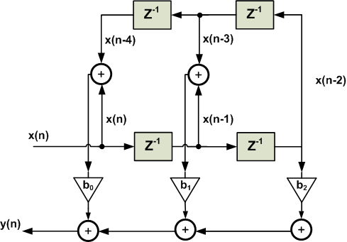
Figure 2. The symmetry of a linear-phase FIR filter can be used to reduce the number of multipliers.

The Cascade-Form Structure

While the direct form is derived from the difference equation, the cascade structure is obtained from the system function $$H(z)$$. The idea is to decompose the target system function into a cascade of second-order FIR systems. In other words, we need to find second-order systems which satisfy

$$H(z)=\sum_{k=0}^{M-1}b_{k}z^{-k}=\prod_{k=1}^{P}\left(b_{0k}+b_{1k}z^{-1}+b_{2k}z^{-2} \right)$$

Equation 2

where $$P$$ is the integer part of $$\tfrac{M}{2}$$. For example, $$M=5$$, $$H(z)$$ will be a polynomial of degree four which can be decomposed into two second-order sections. Each of these second-order filters can be realized using a direct form structure. It is desirable to set a pair of complex-conjugate roots for each of the second-order sections so that the coefficients become real. The reader may wonder why we need to rewrite a given $$H(z)$$ in terms of second-order sections. In a future article, we will see that the main advantage of the cascade structure is its smaller sensitivity to the coefficient quantization.

To clarify converting a system function into the cascade form, let’s review an example.

Example 1

Assume that we need to implement the nine-tap FIR filter given by the following table using a cascade structure.

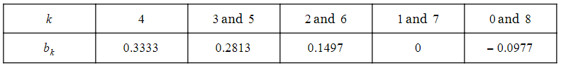
The system function of this filter is

$$H(z)=-0.0977+0.1497z^{-2}+0.2813z^{-3}+0.3333z^{-4}+0.2813z^{-5}+0.1497z^{-6}-0.0977z^{-8}$$

It can be shown that

$$H(z)=GH_{1}(z)H_{2}(z)H_{3}(z)H_{4}(z)$$

where

$$G=-0.0977$$

$$H_{1}(z)=\left(1-2.5321z^{-1}+z^{-2}\right)$$

$$H_{2}(z)=\left(1-0.3474z^{-1}+z^{-2}\right)$$

$$H_{3}(z)=\left(1+1.8794z^{-1}+z^{-2}\right)$$

$$H_{4}(z)=\left(1+z^{-1}+z^{-2}\right)$$

Hence, we obtain the structure shown in Figure 3.

Figure 3. The cascade structure for the system function of Example 1.

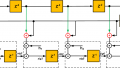
Each of these second-order systems can be realized using the direct-form structure. For example, the realization of $$H_{1}(z)$$ is shown in Figure 4.

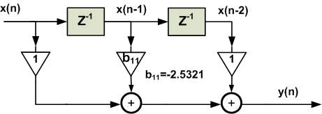
Figure 4. The direct form realization of $$H_{1}(z)$$.

You can verify that $$H_{1}(z)$$ pairs two real zeros of $$H(z)$$, i.e. $$z_1=2.0425$$ and $$z_2=0.4896$$; however, the other three second-order sections (sos) incorporate the complex-conjugate roots of $$H(z)$$. For example, the roots of $$H_2(z)$$ are $$z_3=0.1737 + 0.9848j$$ and $$z_4=0.1737 - 0.9848j$$.

Since finding the cascade form of a practical FIR filter involves tedious mathematics, we can use the MATLAB function tf2sos, which stands for transfer function to second-order section, to obtain the cascade form of a given transfer function. In fact, the cascade form of $$H(z)$$ in the above example was found using the tf2sos function with the following lines of code:

N=[-0.0977 0 0.1497 0.2813 0.3333 0.2813 0.1497 0 -0.0977]; % This line defines the numerator of H(z)

D=1; % This defines the denominator of H(z)

[sos, G]=tf2sos(N, D) % converts the transfer function defined by Nand Dinto a cascade of second-order sections

The result will be:

sos=

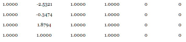
and $$G=-0.0977$$.

Each row of sos above gives the transfer function of one of the second-order sections. The first three numbers of each row represent the numerator of the corresponding second-order section and the second three numbers give its denominator. For example, the first row of sos gives the second-order section $$H_{1}(z)$$ of Example 1 and so on. The tf2sos command also gives a gain factor, $$G$$, which can be included in the cascade-form structure as shown in Figure 3.

Example 2

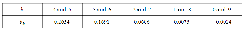
Assume that we need to implement the ten-tap FIR filter given by the following table using a cascade structure.

Similar to the previous example, we have:

N=[-0.0024 0.0073 0.0606 0.1691 0.2654 0.2654 0.1691 0.0606 0.0073 -0.0024];
D=1;
[sos, G]=tf2sos(N, D)

The result will be:

sos =

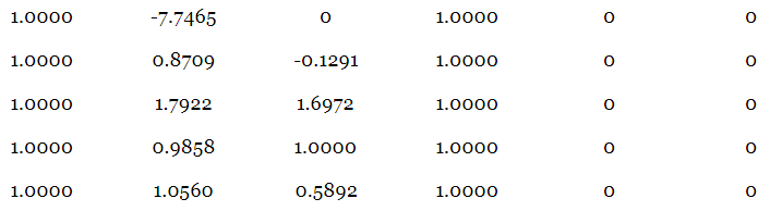
and $$G =-0.0024$$.

Hence, the target system function can be rewritten in terms of second-order sections as

$$H(z)=GH_{1}(z)H_{2}(z)H_{3}(z)H_{4}(z)H_{5}(z)$$

where

$$G=-0.0024$$

$$H_{1}(z)=1-7.7465z^{-1}$$

$$H_{2}(z)=1+0.8709z^{-1}-0.1291z^{-2}$$

$$H_{3}(z)=1+1.7922z^{-1}+1.6972z^{-2}$$

$$H_{4}(z)=1+0.9858z^{-1}+z^{-2}$$

$$H_{5}(z)=1+1.0560z^{-1}+0.5892z^{-2}$$

In this example, the system function polynomial is of degree nine and, hence, the filter has nine zeros. As a result, we observe that $$H_{1}(z)$$ incorporates only one zero, i.e. the coefficient $$b_{2k}$$ in Equation 2 is zero for this second-order section.

We can realize the second-order sections of this example using a direct form structure and obtain the cascade structure of the filter; however, there is another alternative which allows us to reduce the computational complexity. To find this computationally efficient structure, remember that, as illustrated by Figure 1 and 2 above, a linear-phase FIR filter can be realized with a smaller number of multipliers. On the other hand, notice that while the target system function is a linear phase, only $$H_{4}(z)$$ is a linear-phase FIR structure (because of the coefficient symmetry).

So, the question remains: can we group the zeros of a given linear-phase FIR system function in a way that the obtained decomposition incorporates linear-phase structures? For a linear-phase FIR filter, the symmetry in the $$b_{k}$$ coefficients leads to asymmetry in the zeros of the transfer function. In particular, if $$z_{1}$$ and $$z_{1}^{*}$$ are the zeros of the transfer function, then $$\tfrac{1}{z_{1}}$$ and $$\tfrac{1}{z_{1}^{*}}$$ are also a pair of its zeros.We can use this property to group the zeros in a way that the system function is decomposed into linear-phase elements. Let’s use the MATLAB command roots, to find the zeros of the system function:

N=[-0.0024 0.0073 0.0606 0.1691 0.2654 0.2654 0.1691 0.0606 0.0073 -0.0024];

roots(N)

Hence, we obtain:

$$z_1=-1.0000$$

$$z_2=7.7465$$, $$z_3=0.1291$$

$$z_4=-0.4929 + 0.8701j$$, $$z_5=-0.4929 - 0.8701j$$

$$z_6=-0.5280+0.5571j$$, $$z_7=-0.5280-0.5571j$$

$$z_8=-0.8961+0.9456j$$, $$z_9=-0.8961-0.9456j$$

The reader can verify that $$z_2=\tfrac{1}{z_3}$$, $$z_4=\tfrac{1}{z_{5}^{*}}$$, $$z_6=\tfrac{1}{z_{8}^{*}}$$ and $$z_7=\tfrac{1}{z_{9}^{*}}$$. Then, we can pair $$z_2$$ and $$z_3$$ to obtain the following linear-phase second-order section

$$H_{LP1}(z)=(1-0.1291z^{-1})(1-7.7465z^{-1})=(1-7.8756z^{-1}+z^{-2})$$

Pairing $$z_4$$ and $$z_5$$ gives:

$$H_{LP2}(z)=(1-(-0.4929 + 0.8701j)z^{-1})(1-(-0.4929 - 0.8701j)z^{-1})=(1+0.9858z^{-1}+z^{-2})$$

Grouping $$z_6$$, $$z_7$$, $$z_8$$, and $$z_9$$ together, we obtain:

$$H_{LP3}(z)=1+2.8482z^{-1}+4.1790z^{-2}+2.8482z^{-3}+z^{-4}$$

To incorporate the zero $$z_1$$, we need to include a first-order section, i.e. $$H_{LP4}(z)=1+z^{-1}$$. A cascade of these linear-phase elements will give the original system function:

$$H(z)=GH_{LP1}(z)H_{LP2}(z)H_{LP3}(z)H_{LP4}(z)$$

where $$G=-0.0024$$ as before.

In general, the zeros of a linear-phase FIR filter can be of four different arrangements as illustrated in Figure 5. These arrangements include: 1- a pair of complex-conjugate zeros which are not on the unit circle along with their reciprocals, e.g. $$z_1$$, $$z_{1}^{*}$$, $$\tfrac{1}{z_1}$$, and $$\tfrac{1}{z_{1}^{*}}$$ in the figure, 2- a pair of complex-conjugate zeros on the unit circle such as $$z_3$$ and $$z_{3}^{*}$$ in the figure, 3- a real zero which is not on the unit circle along with its reciprocal such as $$z_{2}$$ and $$\tfrac{1}{z_{2}}$$, and finally, 4- a real zero on the unit circle like $$z_4$$ in Figure 5. The system function of the above example had zeros of all these four groups.

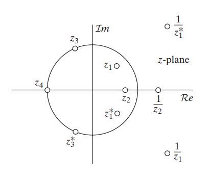
Figure 5. The symmetry of zeros for a linear-phase FIR filter. Image courtesy of Discrete-Time Signal Processing.

Factoring the system function of Example 2 into linear-phase elements, we need a total of five multipliers. The following table shows the number of multipliers for each section.

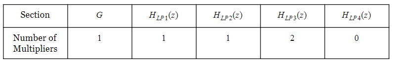
However, the first realization requires nine multipliers as listed below:

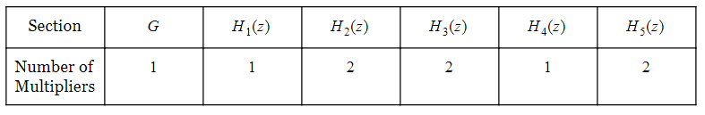
In summary, we can use the tf2sos command to rewrite the system function of a FIR filter as the product of second-order sections; however, these second-order sections are not necessarily linear-phase. To have a cascade of linear-phase elements, we need to group the zeros of the transfer function appropriately. Using a cascade of linear-phase sections, we can reduce the number of multiplications. Note that, in this case, some of the sections might be of order four as $$H_{LP3}(z)$$ in the above example.

Summary

• There are several structures to realize a given system function $$H(z)$$. One consideration choosing the appropriate structure is the sensitivity to coefficient quantization. In addition, sometimes we observe that a particular structure can dramatically reduce the computational complexity of the system.

• The symmetry property of a linear-phase FIR filter can be used to reduce the number of the required multiplications.

• The main advantage of the cascade structure is its smaller sensitivity to the coefficient quantization.

• We can use the tf2sos command to rewrite the system function of a FIR filter as the product of second-order sections; however, these second-order sections are not necessarily linear-phase. To have a cascade of linear-phase elements, we need to group the zeros of the transfer function appropriately.

• ← Previous Article
• Next Article →