Pipelined Direct Form FIR Versus the Transposed Structure

This article will review two pipelined structures to implement a high throughput FIR filter.

This article will review two different structures to implement a high-throughput FIR (finite impulse response) filter: the pipelined direct form FIR and the transposed structure. We’ll see that generally the transposed structure is the preferred implementation for a FIR filter.

Supporting Information

• FIR Filter Design by Windowing: Concepts and the Rectangular Window
• Structures for Implementing Finite Impulse Response Filters
• The Why and How of Pipelining in FPGAs

In a previous article ("Structures for Implementing Finite Impulse Response Filters"), we discussed the direct-form structure of a FIR filter. In the next section, we’ll examine pipelining this structure.

Examining the Direct Form FIR filter

Consider the five-tap FIR filter shown in Figure 1.

 

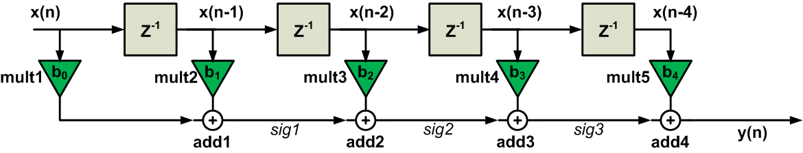
Figure 1. The direct form of a five-tap FIR filter.

 

Let’s see how this circuit processes a new input sample and produces the corresponding output. Assume that multiplication and addition operations introduce a delay of $$T_{mult}$$ and $$T_{add}$$, respectively. All the multipliers of Figure 1 operate simultaneously, for example, when mult1 produces $$x(n)b_0$$, mult5 produces $$x(n-4)b_4$$. Hence, after applying a new input sample, the multipliers will output valid data only after a delay of $$T_{mult}$$ (we assume that the delay of the registers is negligible). Then, we have to wait for add1 to produce a valid output, i.e $$sig1=x(n)b_0+x(n-1)b_1$$. This will introduce an extra delay of $$T_{add}$$. Similarly, each of the remaining additions will have a delay of $$T_{add}$$ and the final output will be produced after a total delay of $$T_{mult}+4T_{add}$$. Hence, the maximum sampling frequency of the filter can be estimated as

 

$$f_{sampling}=\frac{1}{T_{mult}+4T_{add}}$$

Pipelined Direct Form FIR

We can apply the pipelining concept to increase the sampling rate of the circuit in Figure 1. Let’s break the circuit into two cascaded parts (see Figure 2). The delay of Stage 1 is $$T_{mult}+2T_{add}$$. Hence, if the filter takes a new sample at t=0, Stage 1 will produce its valid outputs at $$t=T_{mult}+2T_{add}$$. For $$t > T_{mult}+2T_{add}$$, Stage 1 actually serves no purpose and its outputs won’t change until the filter produces its final output and takes a new sample. This brings us to the idea that we can use some memory elements to store the outputs of Stage 1. These stored values will be applied to the second stage. In this way, Stage 2 will be able to proceed with its calculations meanwhile Stage 1 will be freed to take and process a new input sample. Note that the delay of the two stages are the same in this example.

 

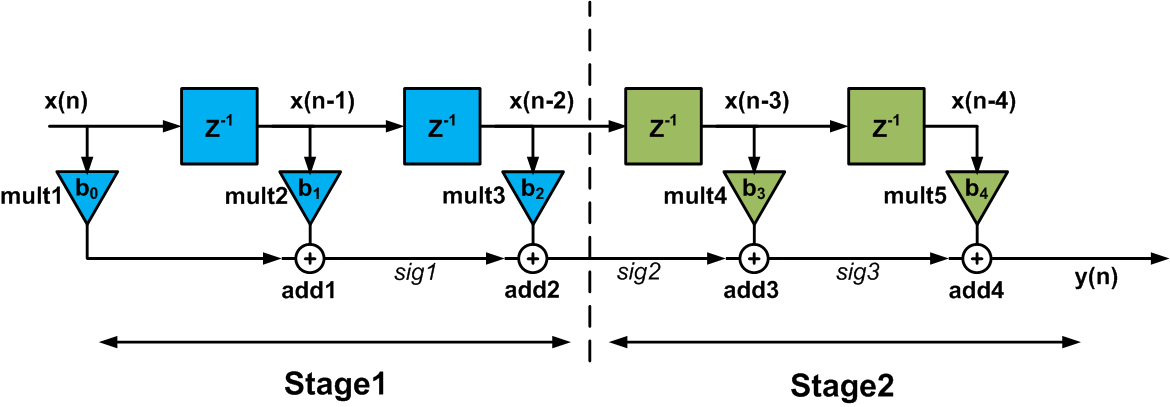
Figure 2

 

Adding pipeline registers at the boundary of the two stages of the circuit, which is shown by the dashed line above, we get the circuit in Figure 3.

 

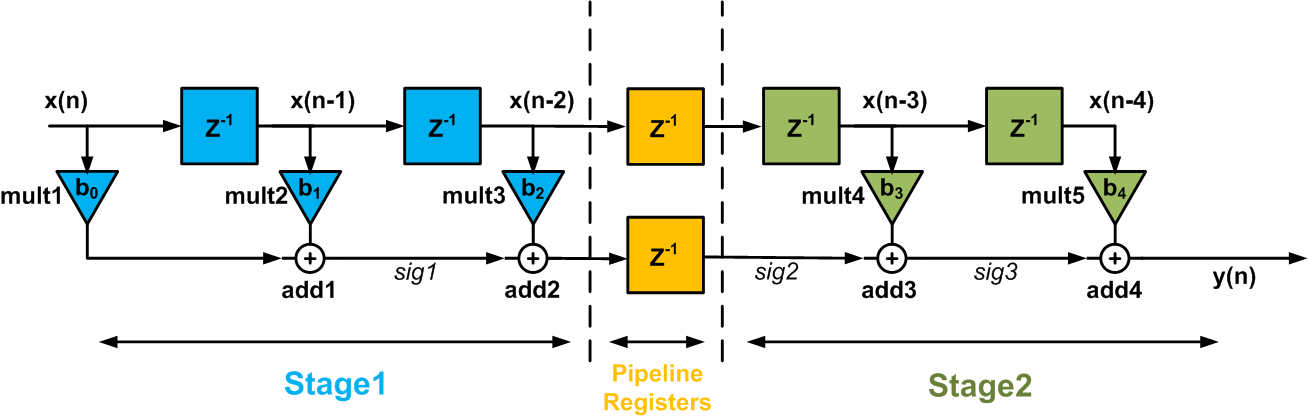
Figure 3

The pipeline registers sample their inputs at the clock edge. Hence, a delay of one clock period will be introduced by the pipeline registers. This delay will be modeled by a unit delay $$z^{-1}$$ in terms of the z transformation.

Now, the “effective critical path” of the circuit will be approximately $$T_{mult}+2T_{add}$$ and the sampling rate of the filter can be increased to

 

$$f_{sampling}=\frac{1}{T_{mult}+2T_{add}}$$

 

Note that, for a general pipelined design, the “critical path” is the longest path among the following paths:

1- The path between any two pipeline registers or

2- Between an input and a pipeline register or

3- Between a pipeline register and an output or

4- Between an input and an output.

 

In the circuit of Figure 3, either the path from input to the pipeline registers or from pipeline registers to the output can be considered as the critical path.

As shown in Figure 4, we can further break the circuit of Figure 3 into smaller stages and obtain a higher sampling rate. In this case, the delay of the critical path will be $$T_{mult}+T_{add}$$ regardless of the number of the filter taps.

 

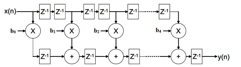
Figure 4. Pipelined direct form FIR. Image courtesy of Xilinx.

Transposed realization of a FIR filter

For a given system, we can achieve a new system structure by applying the “flow graph reversal” or the “transposition” theorem. The new structure is obtained by:

1- reversing the direction of all branches of the original system without changing the function of the branches.

2- reversing the roles of the input and output.

When applying the transposition method, it would be easier to consider the signal flow graph (SFG) of the system. Let’s find the transposed form of Figure 1. The SFG of this system will be as shown in Figure 5.

 

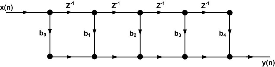
Figure 5

 

Reversing the direction of the branches and the roles of the input and output, we obtain the signal flow graph of Figure 6.

 

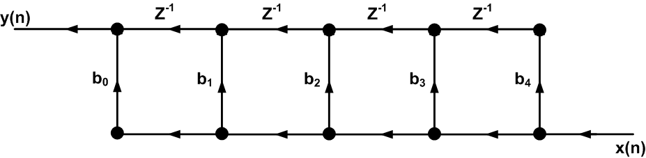
Figure 6

 

Since it is generally convenient to have the inputs on the left and the outputs on the right, we redraw the SFG of Figure 6 as shown in Figure 7.

 

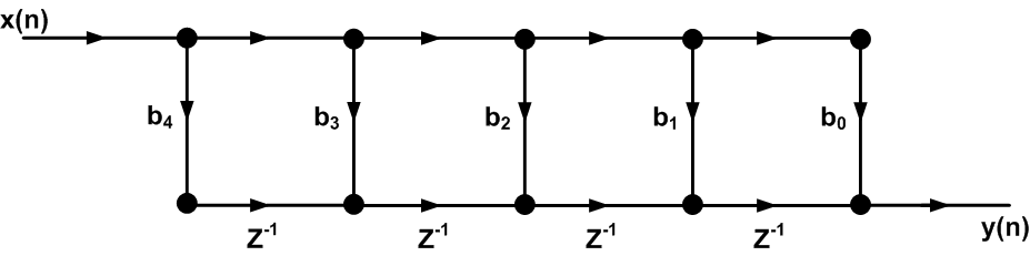
Figure 7. The transposed form of a five-tap FIR filter.

 

The block diagram of the transposed-form FIR is shown in Figure 8.

 

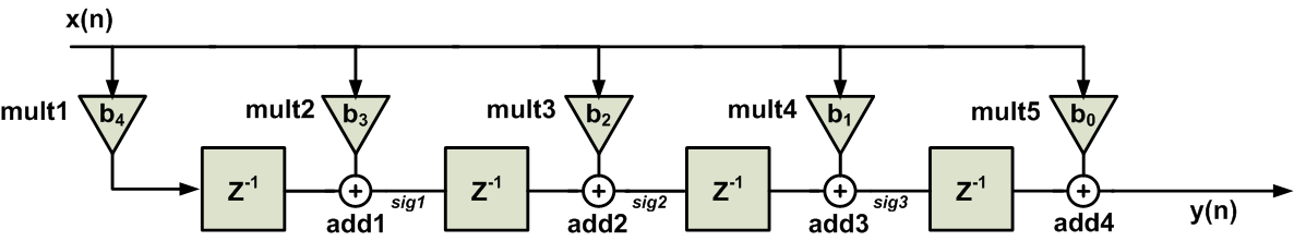
Figure 8

Comparing Figure 8 with the direct form of Figure 1, we observe that the order of the filter coefficients is reversed. Moreover, in the transposed form, the input reaches all of the multipliers at the same time. It is said that the input is broadcast to all of the multipliers. This is in contrast to the direct form structure where a given input sample reaches the multipliers at different clock cycles.

One of the most important features of the new structure is its self-pipelined operation. To understand this, let’s see how a new sample is processed by the transposed structure. We’ll examine the circuit in different clock cycles:

The 1st clock: Assume that, at the first clock edge, a new sample is applied to the filter. After a delay of $$T_{mult}$$, the multiplier mult1 will output $$b_4x(n)$$.

The 2nd clock: At the second clock edge, the output of mult1, which is $$b_4x(n)$$, will be stored in the leftmost register. The register introduces a unit delay, hence, the content of the register will be $$b_4x(n-1)$$. This means that the register stores $$b_4$$ multiplied by the previous sample of the input. To further clarify, note that, we are at the second clock cycle and the stored value corresponds to the sample taken in the first clock cycle.

Besides, with a delay of $$T_{mult}$$, mult2 will output $$b_3$$ times the current input which is $$x(n)$$. Hence, with a delay of $$T_{mult}+T_{add}$$ after the second clock edge, we have $$sig1=b_4x(n-1)+b_3x(n)$$.

The 3rd clock: at the third clock edge, $$sig1=b_4x(n-1)+b_3x(n)$$ will be stored in the corresponding register. Moreover, mult3 will output $$b_2$$ times the current input which is $$x(n)$$. Hence, with a delay of $$T_{mult}+T_{add}$$ after the third clock edge, we have $$sig2=b_4x(n-2)+b_3x(n-1)+b_2x(n)$$.

The 4th clock: with a delay of $$T_{mult}+T_{add}$$ after the fourth clock edge, we have $$sig3=b_4x(n-3)+b_3x(n-2)+b_2x(n-1)+b_1x(n)$$.

The 5th clock: with a delay of $$T_{mult}+T_{add}$$ after the fifth clock edge, we have $$y(n)=b_4x(n-4)+b_3x(n-3)+b_2x(n-2)+b_1x(n-1)+b_0x(n)$$. This is the value of the output during the 5th clock cycle.

What would be the output value during the 6th clock cycle? To answer this question, we can redraw Figure 8 as shown in Figure 9.

 

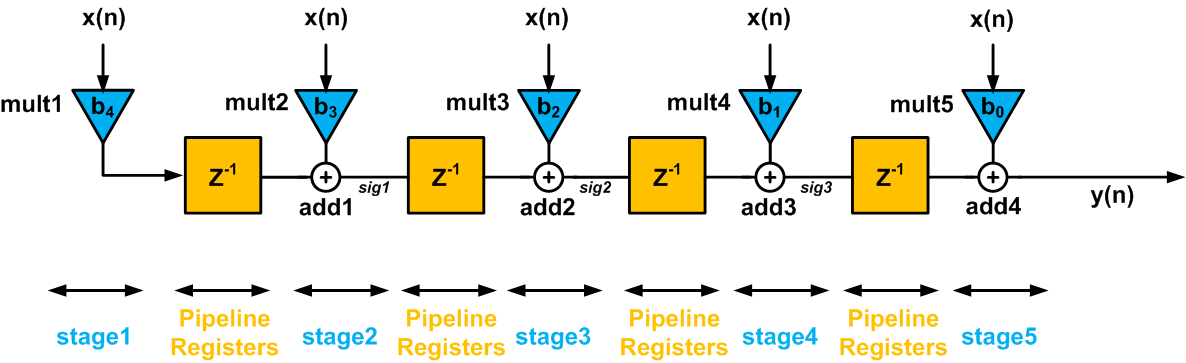
Figure 9

If we consider the transposed structure during different clock cycles, we observe that the registers are storing the final result calculated by all the previous stages. Hence, these previous stages can be used to process new samples. For example, during the second clock cycle discussed above, the leftmost register stores the output of the mult1 multiplier. Hence, mult1 is, in fact, freed to work on the input sample corresponding to the second clock cycle. The result of this calculation will go through the pipeline shown in Figure 9 and, after the steps discussed above, the corresponding output will be produced. As you see, the transposed structure is inherently a pipelined implementation.

Comparison and Conclusion

Let’s compare the transposed structure (Figure 9) to the pipelined direct form FIR shown in Figure 4:

• Both of these two structures are pipelined realizations and offer a high throughput.
• For both Figure 4 and 9, the delay of the critical path is the same and equal to $$T_{mult}+T_{add}$$.
• The transposed structure needs a smaller number of registers.
• Adding pipeline registers to the direct form FIR structure leads to a latency from input to the output but this is not the case for the transposed structure.
• Unlike the pipelined direct form structure, the transposed structure has limitations regarding the fanout of the input. This is due to the fact that the input is broadcast to all of the multipliers. Hence, the fanout of the input must be taken into account when we are designing a filter with a large number of taps.

In summary, considering the number of registers and the latency, the transposed structure is the preferred implementation. However, the pipelined direct form doesn’t have the fanout limitations of the transposed structure.

 

To see a complete list of my articles, please visit this page.