The Effect of Coefficient Quantization on the Performance of a Digital Filter

The previous article in this series discussed some basic structures to implement Finite Impulse Response (FIR) filters. This article will verify that a suitable structure can reduce the sensitivity of the filter response to the coefficient quantization.

For a given set of filter specifications, we generally obtain the filter system function, $$H(z)$$, assuming that the filter coefficients can be represented with infinite precision. However, when implementing the filter in the real world, we have to use a finite number of bits to represent each coefficient of $$H(z)$$. This coefficient quantization can somehow change the location of the filter poles and zeros.

As a result, after implementing a filter, we may observe that the frequency response of the filter is quite different from that of the original design. The error in the pole and zero locations depends on several factors. This article will discuss some of these factors and show how we can design filters which exhibit smaller sensitivity to the coefficient quantization.

Before continuing our discussion, let’s review an example of the coefficient quantization.

Example 1

The transfer function of an Infinite Impulse Response (IIR) filter is given by:

 

$$H(z)=\frac{\sum_{k=0}^{M-1}b_{k}z^{-k}}{\sum_{k=0}^{N-1}a_{k}z^{-k}}$$

 

We can use the MATLAB ellip function to design an elliptic filter. For example, [b, a]=ellip(7,0.5, 50, 0.3) gives a seventh-order elliptic lowpass filter with 0.5 dB ripples in the passband and 50 dB attenuation in the stopband. The passband edge of the filter will be at the normalized frequency of $$0.3 \pi$$. The coefficients of this filter are given in the following table. We will consider these coefficients as the unquantized ones.

 

Table 1. The unquantized coefficients of an elliptic lowpass filter with the passband from DC to $$0.3\pi$$.

k	bk(unquantized)	ak(unquantized)
0	0.012218357882143	1.000000000000000
1	-0.009700754662078	-4.288900601525732
2	0.024350450826845	9.216957436091198
3	0.002532504848041	-12.195350561406707
4	0.002532504848041	10.633166152311462
5	0.024350450826845	-6.062798190498858
6	-0.009700754662078	2.098067018562072
7	0.012218357882143	-0.342340135743532

 

The magnitude of this filter’s frequency response is shown in Figure 1.

 

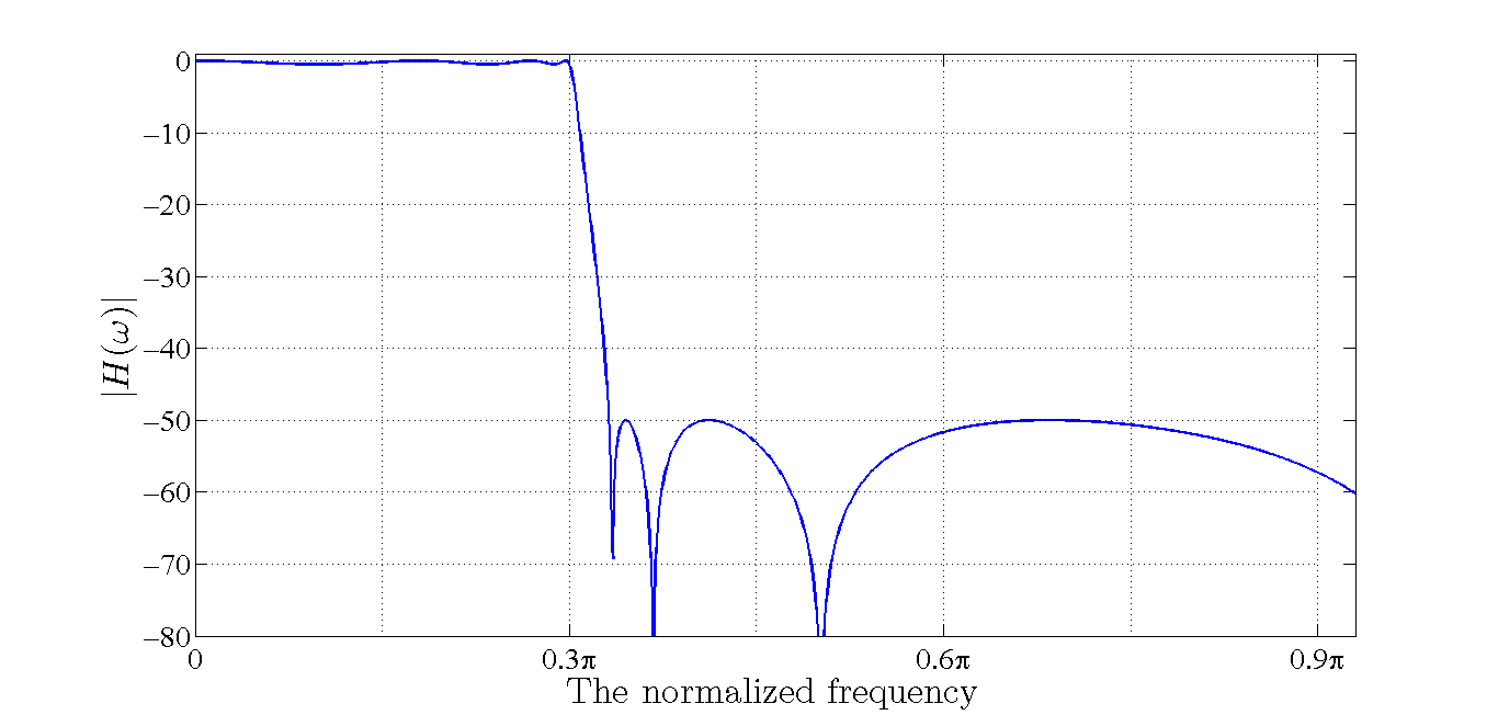
Figure 1. The magnitude of the frequency response of the unquantized filter.

 

Figure 2 shows the poles (blue crosses) and zeros (red dots) of the transfer function. Since the poles are inside the unit circle, the filter is stable.

 

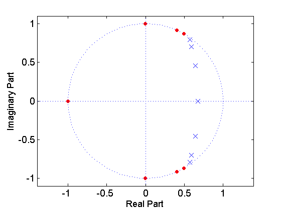
Figure 2. The poles and zeros of the unquantized system function.

We will quantize the coefficients using one bit for the sign and nine bits for the magnitude of the coefficients. Since all the $$b_k$$ coefficients are smaller than $$2^{-5}=0.03125$$, we can consider a scaling factor of $$2^{(number \; of \; bits + 5)}=2^{(9+5)}=16384$$ for these coefficients and achieve a more accurate representation. The quantized $$b_k$$ coefficients are listed in Table 2. For example, to calculate the quantized value of $$b_1$$, we will first apply the scaling factor and obtain:

 

$$b_{1} \times 2^{(9+5)}=0.012218357882143 \times 2^{(9+5)}=200.1856$$

 

Now, we can round the result to $$200$$. The binary representation of $$200$$, which is $$011001000$$, will be used to implement the coefficients. However, we should keep in mind that we need to interpret the results with a rescaling factor of $$2^{-(9+5)}$$. Then, the decimal equivalent of the quantized coefficient can be obtained by multiplying $$200$$ by $$2^{-(9+5)}$$ which gives $$0.0122$$.

In this particular example, with a scaling factor smaller than $$2^{(9+5)}$$, several bits of the binary representation of the $$b_k$$ coefficients would be zero for all the coefficients and we would lose the accuracy. For example, suppose that we allocate nine bits to represent the fractional value of the $$b_k$$ coefficients. Hence, we should apply a scaling factor of $$2^{9}$$ which gives:

 

$$b_{1} \times 2^9=0.012218357882143 \times 2^9=6.2558$$

 

Obviously, in this case, a rescaling factor of $$2^{-9}$$ must be considered when interpreting the result of the calculations. Rounding $$6.2558$$ and converting it to the binary representation, we obtain $$00000110$$. We observe that, although we are using nine bits to represent this number, most of them are zero. The reader can verify that, with this scaling factor, several bits will be zero even for the largest $$b_k$$, i.e. $$0.024350450826845$$.

To quantize the $$a_k$$ coefficients, we note that the magnitude of the integer part of these coefficients is smaller than $$16$$. Hence, we can allocate four bits for the integer part and five bits for the fractional part. As a result, the scaling factor of the $$a_k$$ coefficients will be $$2^5$$. For example, with $$a_2=9.216957436091198$$, we have:

 

$$a_{2} \times 2^5=9.216957436091198 \times 2^5=294.9426 \approx 295$$

 

Hence, the quantized decimal value for the coefficient will be $$9.2188$$. Similarly, we can find the quantized values of other $$a_k$$ coefficients as given in Table 2 below.

 

 

Table 2. The decimal value of the quantized coefficients.

k	bk(quantized)	ak(quantized)
0	0.0122	1.0000
1	-0.0097	-4.2813
2	0.0244	9.2188
3	0.0025	-12.1875
4	0.0025	10.6250
5	0.0244	-6.0625
6	-0.0097	2.0938
7	0.0122	-0.3438

Figure 3 compares the frequency response of the quantized filter (the curve in red) with that of the unquantized system (the curve in blue). We observe that quantizing the coefficients has adversely affected the frequency response.

 

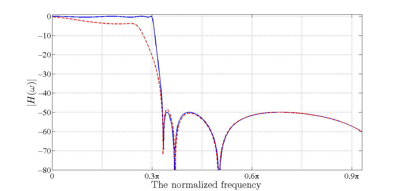
Figure 3. The frequency response of the quantized filter (in red) versus that of the unquantized system (in blue).

 

The poles (blue crosses) and zeros (the red dots) of the quantized filter are shown in Figure 4. As shown in this figure, two of the poles are moved out of the unit circle and the quantized filter is unstable. This example shows that after designing a filter, we need to examine the effect of the coefficient quantization. If the quantized filter does not meet the target specifications, we need to redesign the filter. In the rest of the article, we will see that implementing a high-order filter as a cascade of second-order sections can significantly reduce the sensitivity to the coefficient quantization.

 

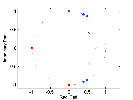
Figure 4. The poles and zeros of the quantized filter.

Analysis of Sensitivity to Coefficient Quantization

To examine the sensitivity of the poles and zeros of a filter to the coefficient quantization, let’s consider a polynomial, $$D(z)$$, with $$N$$ roots:

 

$$D(z)=1+\sum_{k=0}^{N}a_{k}z^{-k}$$

Equation 1

 

Equation 1 can represent the system function of a Finite Impulse Response (FIR) filter or either the numerator or the denominator of an IIR filter. Analyzing the sensitivity of roots of $$D(z)$$ to the coefficient quantization allows us to have a better insight into how the roots and poles of a digital filter will move under finite precision conditions.

We can write $$D(z)$$ in terms of its factors as:

 

$$D(z)=1+\sum_{k=0}^{N}a_{k}z^{-k}=\prod_{k=1}^{N}(1-p_{k}z^{-1})$$

 

Where $$p_k$$ denotes the roots of the polynomial. With a finite number of bits to represent each coefficient, we expect that $$a_k$$ will change to $$a_k+ \Delta a_k$$ where $$\Delta a_k$$ is the error resulted from using a finite precision representation. Consequently, we expect the roots of the polynomial to change from $$p_k$$ to $$p_k+ \Delta p_k$$. The error in the root location, $$\Delta p_i$$, can be found as:

 

$$\Delta p_{i}=-\sum_{k=1}^{N}\frac{p_{i}^{N-k}}{\prod_{l=1, l \neq i}^{N}(p_{i}-p_{l})}\Delta a_{k}$$

Equation 2

 

To see the proof of Equation 2 refer to section 9.5 of this book. Equation 2 has two important implications that will be discussed next.

Avoid Clusters of Poles and Zeros

Firstly, the error in the $$i$$th root, $$\Delta p_i$$, is equal to the error in the $$k$$th coefficient multiplied by the following factor:

 

$$F_{k}=\frac{p_{i}^{N-k}}{\prod_{l=1, l \neq i}^{N}(p_{i}-p_{l})}$$

Equation 3

 

This factor can be very large when the polynomial has other roots close to the $$i$$th pole, i.e. $$p_{i}-p_{l}$$ is small. In other words, when we have a cluster of roots, the error in the root locations will be much higher for a given $$\Delta a_k$$. Since a narrow band filter has generally tightly clustered roots, we expect that the frequency response of these filters will be highly sensitive to the coefficient quantization.

Avoid High-Order Filter Sections

Rewriting Equation 2 as Equation 4 below, we observe that each and every coefficient of the polynomial contributes some error to the location of a particular pole:

 

$$\Delta p_{i}=-\sum_{k=1}^{N}F_{k}\Delta a_{k}$$

Equation 4

 

This means that as the number of roots of a polynomial increases, the sensitivity to the quantization error will increase. This is due to the fact that each root of $$D(z)$$ in Equation 1 depends on the value of all the coefficients $$a_{k}$$. For a polynomial of degree $$N$$, there are $$N$$ coefficients that need to be quantized. And, obviously, each of these quantized coefficients will contribute a particular amount of error to the overall error.

To summarize, we should avoid clusters of poles and zeros and use low-order filter sections. These two goals can be achieved by using single-pole sections to implement a high-order filter. However, a filter has generally complex poles and zeros and use of single-pole sections mandates complex arithmetic which increases the computational complexity. The next best alternative is to use second-order sections. In this case, we can pair complex-conjugate roots and avoid the complex arithmetic. Since finding the cascade form of a high-order filter involves tedious mathematics, we can use the MATLAB function tf2sos, which stands for transfer function to second-order section, to obtain the cascade form of a given transfer function.

Example 2

We will use the tf2sos function to convert the transfer function of Example 1 into the cascade form. Then we will quantize the coefficients of these second-order sections and compare the frequency response of the obtained structure with that of the unquantized system.

The following lines of code define the transfer function of Example 1 and convert that to second-order sections:

 

N=[0.012218357882143  -0.009700754662078   0.024350450826845   0.002532504848041   0.002532504848041   0.024350450826845  -0.009700754662078  0.012218357882143]; % This line defines the numerator of H(z)

D=[1.000000000000000  -4.288900601525731   9.216957436091192 -12.195350561406695  10.633166152311450  -6.062798190498850   2.098067018562069 -0.342340135743531]; % This defines the denominator of H(z)

[sos, G]=tf2sos(N, D) % converts the transfer function defined by N and D into a cascade of second-order sections

 

The result will be:

 

sos =

1.0000000000	1.0000000000	0.0000000000	1.0000000000	-0.6790830001	0.0000000000
1.0000000000	0.0102799961	1.0000000000	1.0000000000	-1.2818759037	0.6209275764
1.0000000000	-0.8106030432	1.0000000000	1.0000000000	-1.1804902667	0.8437961219
1.0000000000	-0.9936260871	1.0000000000	1.0000000000	-1.1474514311	0.9621803579

 

and:

 

$$G=$$0.0122183579.

Each row of sos above gives the transfer function of one of the second-order sections. The first three numbers of each row represent the numerator of the corresponding second-order section and the second three numbers give its denominator. For example, the second-order section obtained from the second row is:

 

$$H_{2}(z)=\frac{1.0000000000+0.0102799961z^{-1}+1.0000000000z^{-2}}{1.0000000000-1.2818759037z^{-1}+0.6209275764z^{-2}}$$

 

We will quantize the coefficients using one bit for the sign and nine bits for the magnitude of the coefficients. We need to choose an appropriate scaling factor. Since the coefficients of the second-order sections are less than 2, we will use one bit for the integer part and eight bit for the fractional part, i.e. the scaling factor will be $$2^8$$. Hence, we obtain the transfer function of the first section as:

 

$$H_{1}(z)=\frac{1.00000000+1.00000000z^{-1}}{1.00000000-0.67968750z^{-1}}$$

 

The quantized transfer function of the other second-order sections will be:

 

$$H_{2}(z)=\frac{1.00000000+ 0.01171875z^{-1}+1.00000000z^{-2}}{1.00000000-1.28125000z^{-1}+ 0.62109375z^{-2}}$$

$$H_{3}(z)=\frac{1.00000000-0.81250000z^{-1}+1.00000000z^{-2}}{1.00000000-1.17968750z^{-1}+0.84375000z^{-2}}$$

$$H_{4}(z)=\frac{1.00000000-0.99218750z^{-1}+1.00000000z^{-2}}{1.00000000-1.14843750z^{-1}+0.96093750z^{-2}}$$

 

Figure 5 compares the frequency response of $$H(z)=GH_{1}(z)H_{2}(z)H_{3}(z)H_{4}(z)$$ (which is shown in red) with that of the unquantized filter (shown in blue). As you can see the two graphs are barely distinguishable from each other.

 

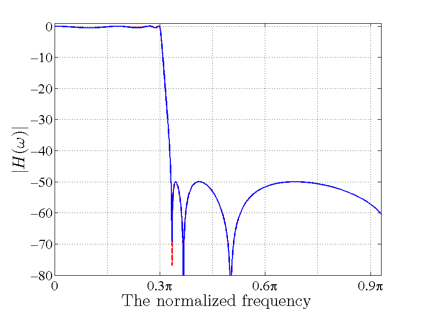
Figure 5. The frequency response of the cascade structure (in red) versus that of the unquantized system (in blue).

 

The reader can easily use MATLAB roots() function to verify that the poles of the quantized cascade structure are inside the unit circle and the system is stable. This example shows that implementing a high-order filter as a cascade of second-order sections can significantly reduce the sensitivity to the coefficient quantization.

Summary

• When implementing a digital filter in the real world, we have to use a finite number of bits to represent each coefficient of $$H(z)$$.
• The frequency response of the quantized filter might be quite different from that of the original design.
• Implementing a high-order filter as a cascade of second-order sections can significantly reduce the sensitivity to the coefficient quantization.

Supporting Information

• ← Previous Article

• FIR Filter Design by Windowing: Concepts and the Rectangular Window
• Undesired Effects of a Window Function in FIR Filter Design
• The Bartlett Versus the Rectangular Window
• From Filter Specs to Window Parameters in FIR Filter Design
• Design of FIR Filters Using the Frequency Sampling Method
• Structures for Implementing Finite Impulse Response Filters