The Polyphase Implementation of Interpolation Filters in Digital Signal Processing

This article discusses an efficient implementation of the interpolation filters called the polyphase implementation.

In digital signal processing (DSP), we commonly use the multirate concept to make a system, such as an A/D or D/A converter, more efficient. This article discusses an efficient implementation of one of the main building blocks of the multirate systems, the interpolation filter. The method we'll cover here is called the polyphase implementation.

We can derive the polyphase implementation of the decimation and interpolation systems using the frequency-domain representation of the signals and systems. This is outside the scope of this article, but you can learn more in section 11.5 of the book Digital Signal Processing by John Proakis.

Here, we will attempt to clarify the operation of a polyphase interpolation filter examining a specific example in time-domain.

Interpolation

As shown in Figure 1, the straightforward implementation of interpolation uses an upsampler by a factor of $$L$$ and, then, applies a lowpass filter with a normalized cutoff frequency of $$\frac{\pi}{L}$$. You can read about the interpolation filter in my article, Multirate DSP and Its Application in D/A Conversion.

 

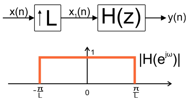
Figure 1. Upsampling followed by a low-pass filter with a normalized cutoff frequency of Lperforms interpolation.

 

The upsampler places $$L-1$$ zero-valued samples between adjacent samples of the input, $$x(n)$$, and increases the sample rate by a factor of $$L$$. Hence, the filter in Figure 1 is placed at the part of the system which has a higher sample rate.

A finite impulse response filter (FIR) of length $$N$$ which is placed before the upsampler needs to perform $$N$$ multiplications and $$N-1$$ additions for each sample of $$x(n)$$. However, the filter of Figure 1, which is placed after the upsampler, will have to perform $$LN$$ multiplications and $$L(N-1)$$ additions for each sample of $$x(n)$$.

Is there any way to relax the computational complexity of this system?

To answer this question, we need to note that while the filter realizing $$H(z)$$ in Figure 1 is clocked at a higher sample rate, $$L-1$$ samples out of every $$L$$ samples that $$H(z)$$ processes are zero-valued. Hence, for $$L=2$$ at least $$50$$% of the input samples of $$H(z)$$ are zero-valued. This percentage will increase even further for $$L>2$$.

Considering the fact that multiplying a filter coefficient by a zero-valued input leads to a zero-valued product, we may be able to decrease the computational complexity of the system in Figure 1. To get a better insight, let’s investigate a simple example of interpolation where $$L=2$$.

Interpolation with $$L=2$$

Let’s assume that $$L=2$$ and $$H(z)$$ is an FIR filter of length six with the following difference equation:

 

$$y(n)=\sum_{k=0}^{5}b_{k}x(n-k)$$

Equation 1

 

Assume that the input signal, $$x(n)$$, is as shown in Figure 2.

 

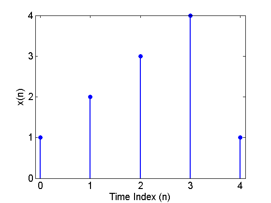
Figure 2. The input sequence $$x(n)$$.

 

After upsampling by a factor of two, we have $$x_1(m)$$ shown in Figure 3 below:

 

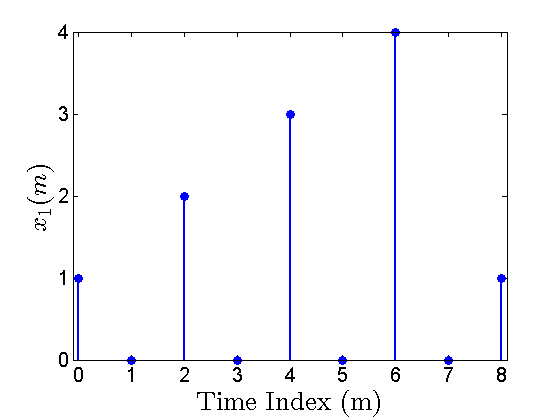
Figure 3. The upsampled sequence $$x_1(m)$$.

Assume that the six-tap FIR filter is implemented with the direct-form structure below:

 

 

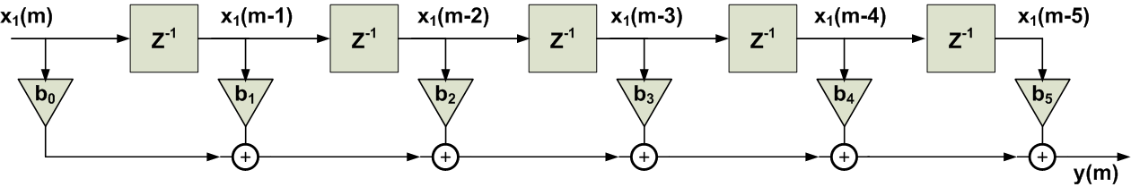
Figure 4. The direct-form realization of a six-tap FIR filter.

 

With these assumptions, let’s examine the straightforward implementation of the interpolation filter in Figure 1. At time index $$m=5$$, the FIR filter will be as shown in Figure 5.

 

 

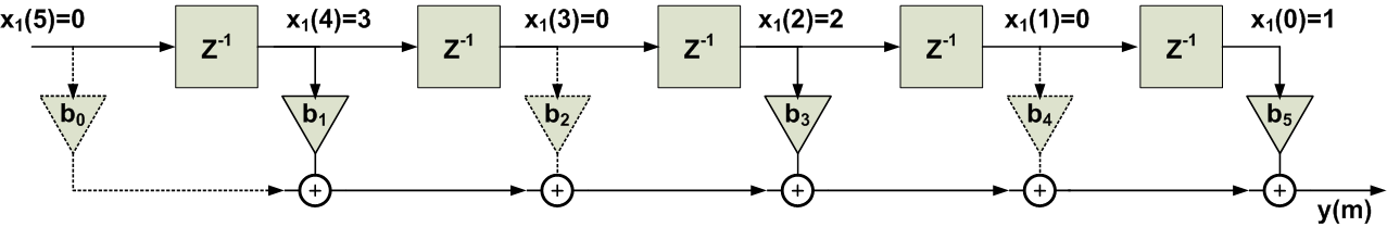
Figure 5. The FIR filter at $$m=5$$.

 

As you can see, at $$m=5$$, half of the multiplications of the FIR filter have a zero-valued input. The branches corresponding to these multiplications are shown by the dashed lines. You can verify that, for an odd, these multiplications will be always zero and $$y(m)$$ will be determined only by the coefficients $$b_1$$, $$b_3$$, and $$b_5$$. At the next time index, i.e. $$m=6$$, we obtain Figure 6 below:

 

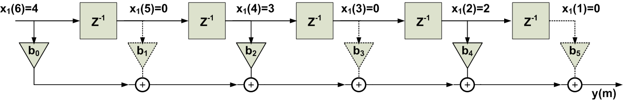
Figure 6. The FIR filter at m=6.

Again those branches which incorporate a zero-valued input are shown by dashed lines. Figure 6 shows that, again, half of the multiplications have a zero-valued input. Examining Figures 5 and 6, we observe that, for an odd time index, half of the coefficients, namely $$b_1$$, $$b_3$$, and $$b_5$$, determine the output value and the sum of the products incorporating the other coefficients is zero. For an even time index, the coefficients, i.e. $$b_0$$, $$b_2$$, and $$b_4$$, are important and the sum of the products for the rest of the coefficients becomes zero.

Let’s use two different filters after the upsampler: one with the odd coefficients and the other one with the even coefficients and add the output of these two filters together to get $$y(m)$$. The result is shown in Figure 7.

 

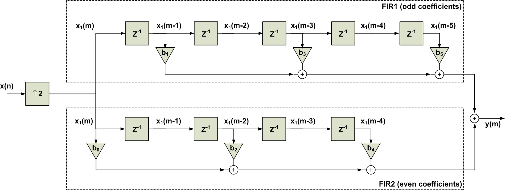
Figure 7. Breaking the Filter’s difference equation into two sets of coefficients: the odd coefficients and the even ones.

 

We can easily obtain the above figure by manipulating Equation 1 as

 

$$y(n)= \big ( b_0 x(n)+ b_2 x(n-2) + b_4 x(n-4) \big ) + \big ( b_1 x(n-1)+ b_3 x(n-3) + b_5 x(n-5) \big )$$

Equation 2

 

However, our previous discussion shows why we are interested in this decomposition: at each time index, only one of these two filters can produce a non-zero output and the other one outputs zero. To further clarify, let’s consider the lower path of Figure 7. We know that the output of this path is non-zero only for even time indexes. As a result, we only need to simplify the cascade of the upsampler and FIR2 at even time indexes where the filter output is non-zero.  At the next time index, we can simply connect the output of the path to zero. This will be further explained in the rest of the article.

Now, let’s examine the upsampler followed by the lower path of Figure 7 which incorporates the even coefficients. In this path, we are first upsampling the input $$x(n)$$ to obtain $$x_1(m)$$. With this operation, as shown in Figures 2 and 3, we are creating a time difference equal to two time units between every two successive samples of $$x(n)$$. On the other hand, the filter FIR2 in Figure 7, “looks” at its input at multiples of “two time units”. For example, while the multiplication by $$b_0$$ takes the current sample, multiplications by $$b_2$$ and $$b_4$$ are receiving samples with two time units and four time units distances, respectively. Therefore, when the output of FIR2 is going to be non-zero, we can simply find the output by applying $$x(n)$$ rather than $$x_1(m)$$ to the coefficients $$b_0$$, $$b_2$$, and $$b_4$$ provided that we are using a delay of one unit time, i.e. $$Z^{-1}$$, between these coefficients. This equivalent filtering is shown in Figure 8.

 

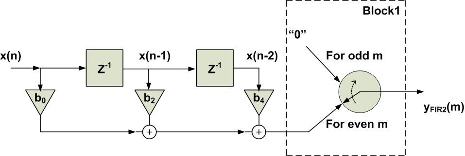
Figure 8. The schematic is equivalent to the cascade of the upsampler and FIR2 in Figure 7.

 

Figure 8 also includes a switch after the filter, why do we need this switch? Remember that FIR2 in Figure 7 has a non-zero output for an even $$m$$. For an odd $$m$$, the output of this filter will be always zero in our example. That’s why we need to force the output of the equivalent circuit in Figure 8 to be zero for an odd m. Interestingly, the operation of this particular switch is exactly the same as that of an upsampler by a factor of two. Hence, we obtain the final equivalent schematic in Figure 9.

 

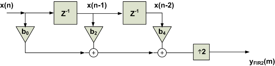
Figure 9. The schematic is equivalent to the cascade of upsampler and FIR2 in Figure 7.

What is the advantage of Figure 9 over the cascade of the upsampler and FIR2 in Figure 7? In Figure 7, we were evaluating FIR2 at both the odd and even time indexes regardless of the fact that, for an odd time index, the output of FIR2 is always zero. In Figures 8 and 9, this property is taken into account and the output is directly connected to zero for an odd time index. In this way, we are avoiding unnecessary calculations. In other words, the three-tap FIR filter in Figure 9 is placed before the upsampler, hence, we only perform three multiplications and two additions for each input sample of x(n). However, the lower path of Figure 7 places the multiplications after the upsampler and we would have to perform six multiplications and four additions for each input sample of $$x(n)$$.

The process of simplifying the lower path of Figure 7 to the block diagram in Figure 9 is actually a particular example of an identity called the second noble identity. This identity is shown in Figure 10.

 

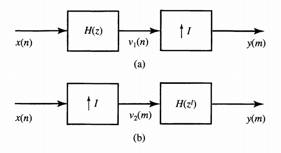
Figure 10. The second noble identity states that these two systems are equivalent. Image courtesy of Digital Signal Processing.

 

Considering our previous discussion, you should now be able to imagine why we are allowed to bring a system which can be expressed in terms of ZI, i.e. H(ZI), before the factor-of-I upsampler provided that, for the new system, ZIis replaced by Zin the transfer function. In fact, the upsampler creates a time difference equal to I time units between every two successive samples of x(n). However, for a time index at which the output is non-zero, the system function H(ZI) “looks” at its input at multiples of “I time units”. Hence, we can simplify the cascade of the upsampler and the system function in manner similar to what we did with the FIR2 path in Figure 7.  To read about the proof of the second noble identity read Section 11.5.2 of this book.

How can we simplify the upper path of Figure 7? We can obtain the system function FIR1 as

 

$$H_{FIR1}(z)=b_{1}z^{-1}+b_{3}z^{-3}+b_{5}z^{-5}$$

 

To use the second noble identity, we only need to express this function in terms of $$z^{-2}$$. We can rewrite the system function as

 

$$H_{FIR1}(z)=\big ( b_{1}+b_{3}z^{-2}+b_{5}z^{-4} \big ) z^{-1} = P_{1}(z^{2})z^{-1}$$

 

Since $$P_1(z^2)$$ is in terms of $$z^2$$, we can use the noble identity to move this part of the transfer function before the upsampler. In this case, we will have to replace $$z^2$$ with $$z$$ in $$P_1(z^2)$$. The final system is shown in Figure 11.

 

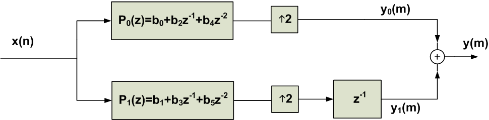
Figure 11. The final system obtained after applying the second noble identity.

 

In this system, all of the multiplications are performed before the upsampling operations. Hence, a significant reduction in the computational complexity is achieved. The schematic of Figure 11 is called the polyphase implementation of the interpolation filter.

Now, let’s examine the general form of the above example. In this case, we have a factor-of-M upsampler followed by a system function H(z).

Polyphase Decomposition and Efficient Implementation of an Interpolator

To find the M-component polyphase decomposition of a given system $$H(z)$$, we need to rewrite the system function as

 

$$H(z)=\sum_{k=0}^{M-1}z^{-k} P_{k}(z^M)$$

Equation 3

 

where $$P_k(z)$$ is called a polyphase component of $$H(z)$$ which is given by

 

$$P_{k}(z)=\sum_{n=-\infty}^{+\infty}h(nM+k)z^{-n}$$

Equation 4

 

Now, if $$H(z)$$ is preceded by a factor-of-M upsampler, we can apply the second noble identity to $$P_k(z^M)$$ components and achieve a more efficient implementation.

For example, if H(z)is preceded by a factor-of-3 upsampler, we can use the decomposition of Equation 2 to obtain Figure 12 below.  we will obtain Figure 12 for M=3. Now, applying the second noble identity, we will have Figure 13. To get more comfortable with Equations 2 and 3, try using these two equations to obtain the schematic of Figure 11 directly from the system function of the filter in Equation 1.

 

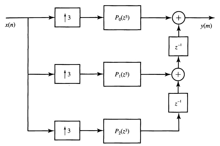
Figure 12. The three-component polyphase decomposition of $$H(z)$$ preceded by a factor-of-three upsampler. Image courtesy of Digital Signal Processing.

 

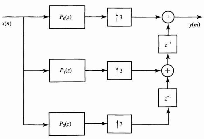
Figure 13. Use of the three-component polyphase decomposition of $$H(z)$$ to implement the factor-of-three upsampler followed by $$H(z)$$. Image courtesy of Digital Signal Processing. 

 

For more details and examples see Section 11.5 of Digital Signal Processing, Section 12.2 of Digital Signal Processing: Fundamentals and Applications, and also this excellent paper from IEEE.

Summary

• The straightforward implementation of the interpolation filter places $$H(z)$$ at the part of the system which has a higher sample rate.
• A finite impulse response (FIR) filter of length $$N$$ which is placed before the upsampler needs to perform $$N$$ multiplications and $$N-1$$ additions for each sample of $$x(n)$$. However, the filter of Figure 1, which is placed after the upsampler, will have to perform $$LN$$ multiplications and $$L(N-1)$$ additions for each sample of $$x(n)$$.
• According to the second noble identity, we are allowed to bring a system which can be expressed in terms of $$Z^I$$, i.e., $$H(Z^I)$$, before the factor-of-I upsampler provided that, for the new system, $$Z^I$$ is replaced by $$Z$$ in the transfer function.
• If $$H(z)$$ is preceded by a factor-of-M upsampler, we can rewrite the system function in terms of its polyphase components, $$P_k(z^M)$$, and apply the second noble identity to swap the position of the polyphase components and the upsampler.

To see a complete list of my DSP-related articles on AAC, please see this page.