Facebook
 Google
 GitHub
 Linkedin
Digital Signal Processing in Scilab: How to Remove Noise in Recordings with Audio Processing Filters
This article is an introduction to the complex topic of DSP-based reduction of noise in audio signals.
This article is an introduction to the complex topic of DSP-based reduction of noise in audio signals.
Scientists and engineers have dedicated countless hours to the pursuit of high-quality audio. Sound happens so naturally in the biological world, and it is really rather astonishing to think of the extreme difficulty involved in recording sound and playing it back without introducing noticeable degradation.
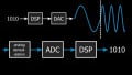
Optimizing audio quality is something that must occur throughout the system—from the microphone to the speaker and everything in between. In this article, we’ll look at the DSP block, where digitized audio signals are modified by means of carefully designed algorithms. This is just one portion of the audio signal chain, but it’s a very important portion because digital signal processing is so versatile and can mitigate imperfections introduced by other components.
Before moving on, please check out these resources for context and related info:
Supporting Information
-
Learning to Live in the Frequency Domain (from Chapter 1 of AAC’s RF textbook)
Related Information
- An Introduction to Audio Electronics: Sound, Microphones, Speakers, and Amplifiers
- Addressing Harmonic Distortion in Audio Amplifiers
- My 40-Year Love Affair with a Remarkable Amplifier—A Class B Amplifier for Audiophiles
Previous Articles on Scilab-Based Digital Signal Processing
- Introduction to Sinusoidal Signal Processing with Scilab
- How to Perform Frequency-Domain Analysis with Scilab
- How to Use Scilab to Analyze Amplitude-Modulated RF Signals
- How to Use Scilab to Analyze Frequency-Modulated RF Signals
- How to Perform Frequency Modulation with a Digitized Audio Signal
Reducing Hiss
The goal of this article is to remove the background noise found in a recording of a person’s voice. The sort of noise that I’m talking about is called “hiss,” and it’s much easier to explain with an example than with words. The following audio file is a recording of me reading the first two lines of “The Raven” by Edgar Allen Poe. Hiss is present throughout the recording, and it’s especially noticeable at the end after I stop speaking.
Significantly reducing hiss is not a simple task. In this article, we’ll use filters, which are straightforward but not particularly effective.
Loading and Analyzing the Audio File
The following command will convert your WAV file into Scilab variables:
[OriginalAudio, Fs] = wavread("C:\Users\Robert\Documents\Audio\OnceUponaMidnightDreary.wav");
If you’ve read How to Perform Frequency Modulation with a Digitized Audio Signal, you’re familiar with the wavread() command. You may have noticed that this version is a bit different, though. If you include two return variables, the second one will contain the audio file’s sample rate. This is handy, because we know from previous articles that discrete-time frequency-domain analysis requires knowledge of the sample rate.
You can use the following command to confirm that your recording sounds correct:
playsnd(OriginalAudio, Fs)
Now let’s take a look at the spectral characteristics of the audio signal. We could, of course, use the fft() command and then plot the data according to the procedure presented in a previous article. However, we can simplify our lives a bit by taking advantage of Scilab’s analyze() command. If you give this function an array representing a digitized signal along with the signal’s sample rate, it will generate a frequency-domain plot that already has the horizontal axis set up to display frequency in hertz; you also specify the minimum and maximum frequency to be displayed and the number of samples. For example:
Fmin = 20;
Fmax = 20e3;
analyze(OriginalAudio, Fmin, Fmax, Fs, length(OriginalAudio))

Fmax = 2e3;
analyze(OriginalAudio, Fmin, Fmax, Fs, length(OriginalAudio))

Analyzing the Hiss
The plan here is to use a filter to reduce the hiss. The filter must be designed according to the frequency content of the hiss, and we can determine this frequency content by looking at the spectrum of an audio excerpt that has only background noise. In my file, I stop speaking at approximately 9 seconds, and the recording ends a little after 12 seconds. So let’s extract the data corresponding to the audio from 10 seconds to 12 seconds and then look at the frequency-domain plot.
Fmax = 20e3;
OriginalAudio_NoiseOnly = OriginalAudio(10*Fs : 12*Fs);
playsnd(OriginalAudio_NoiseOnly, Fs)     // to confirm that the excerpt contains only background noise
analyze(OriginalAudio_NoiseOnly, Fmin, Fmax, Fs, length(OriginalAudio_NoiseOnly))

Fmax = 1e3;
analyze(OriginalAudio_NoiseOnly, Fmin, Fmax, Fs, length(OriginalAudio_NoiseOnly))

As you can see, the background noise has fairly constant amplitude over a wide range of frequencies and higher amplitude within a small band below 100 Hz. There is also a relatively high-amplitude noise component at 60 Hz; I’m in North America and my audio system is surrounded by 60 Hz power, so this confirms that the analyze() command is giving us accurate frequency information.
Designing and Implementing the Filter
For this task, we will use Scilab’s graphical FIR filter design tool.
FIR_coefficients = wfir();
Unfortunately, there isn’t a lot that we can accomplish with ordinary filtering. I don’t think it’s a good idea to try to filter out the low-frequency noise or the 60 Hz spike, because the original signal has a large spectral component centered at about 80 Hz. We can certainly do some low-pass filtering, but we have to decide where to place the cutoff frequency.
When I look at the spectrum of the original signal, I get the impression that the noise makes a dominant contribution starting at about 5 kHz.


After you click OK, the coefficients are stored in the FIR_coefficients variable, and then we can apply the filter via convolution. For this we use the convol() command.
FilteredAudio = convol(FIR_coefficients, OriginalAudio);
analyze(FilteredAudio, Fmin, Fmax, Fs, length(FilteredAudio))

You can see that we have successfully suppressed the higher-frequency content. Here’s the resulting audio:
I think that the volume of the hiss has diminished, though the results are far from impressive—the hiss is still very noticeable and the quality of the voice has been altered. It seems more flat and distant—more like a recording and less like real life. I suppose that’s not surprising since some of the subtle characteristics of the sound were lost when we removed those higher frequencies.
The following two recordings give you an idea of how the audio quality is affected by a higher or lower cutoff frequency (fC).
fC = 7 kHz
fC = 3 kHz
Conclusion
In this article, we investigated the noise characteristics of a typical voice recording and attempted to improve the audio quality using a low-pass filter. If you have any ideas about how to achieve superior hiss reduction using filters, please share your thoughts in the comments section below.