Digital Signal Processing in Scilab: How to Decode an FSK Signal

Learn about a DSP technique that extracts the original digital data from a demodulated frequency-shift-keying baseband signal.

Related Information

• Digital Modulation: Amplitude and Frequency (from Chapter 4 of AAC’s RF textbook)
• How to Demodulate Digital Phase Modulation

Previous Articles on Scilab-Based Digital Signal Processing

• Introduction to Sinusoidal Signal Processing with Scilab
• How to Perform Frequency-Domain Analysis with Scilab
• How to Use Scilab to Analyze Amplitude-Modulated RF Signals
• How to Use Scilab to Analyze Frequency-Modulated RF Signals
• How to Perform Frequency Modulation with a Digitized Audio Signal
• Digital Signal Processing in Scilab: How to Remove Noise in Recordings with Audio Processing Filters
• Audio Processing in Scilab: How to Implement Spectrum Subtraction

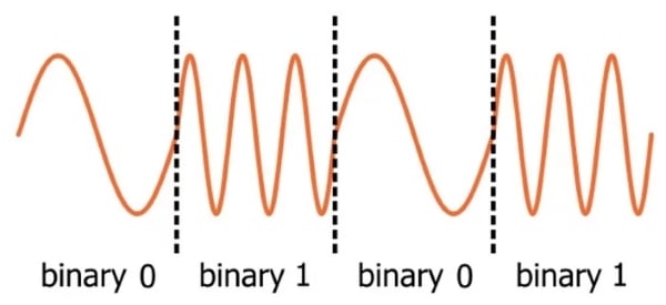
One of the methods used to encode binary data in a sinusoidal waveform is called frequency shift keying (FSK). It’s a simple concept: one frequency represents a zero, and a different frequency represents a one. For example:

 

 

A low-frequency FSK signal (say, in the tens of kilohertz) can be shifted to a higher frequency and then transmitted. This is an effective and fairly straightforward way to create an RF system that achieves wireless transmission of digital data—assuming that we have a receiver that can convert all these sinusoidal waveforms back into ones and zeros.

The process of extracting digital data from a transmitted FSK signal can be divided into two general tasks: First, the high-frequency received signal is converted to a low-frequency baseband signal. I refer to this as “demodulation.” Second, the baseband waveform must be converted into ones and zeros. I don’t think that it would be incorrect to call this second step “demodulation,” but to avoid confusion I’ll always use the term “decoding” when I’m talking about converting lower-frequency analog waveforms to digital bits.

 

Decoding in Software

For systems with moderate data rates, it is perfectly feasible to digitize an FSK baseband signal and perform decoding in software. (You can check out our introduction to software-defined radio for more information on RF systems that implement important signal-processing tasks in software.) This is an excellent approach, in my opinion, because it allows the receiver to benefit from the versatility of digital signal processing, and it also provides a convenient way to record and analyze received signals during testing.

In this article, we’ll use Scilab to decode an FSK signal, but the computations involved are not complicated and could easily be implemented as C code in a digital signal processor.

First Things First: The Math

Our technique for decoding FSK is based on the multiplication of sinusoidal signals. Consider the following trigonometric identities:

 

$$\sin(x)*\sin(y)=\frac{1}{2}(\cos(x-y)-\cos(x+y))$$

$$\cos(x)*\cos(y)=\frac{1}{2}(\cos(x-y)+\cos(x+y))$$

 

Let’s make this more consistent with the engineering world by using ω₁t and ω₂t instead of x and y.

 

$$\sin(\omega_1t)*\sin(\omega_2t)=\frac{1}{2}(\cos((\omega_1-\omega_2)t)-\cos((\omega_1+\omega_2)t))$$

$$\cos(\omega_1t)*\cos(\omega_2t)=\frac{1}{2}(\cos((\omega_1-\omega_2)t)+\cos((\omega_1+\omega_2)t))$$

 

(Note that we are ignoring the effect of phase differences; in this article we’re assuming that all the signals have equal phase.) We can multiply two sine waves or two cosine waves, and the result consists of two cosine waves, with frequencies equal to the sum and the difference of the two original frequencies. The critical observation here is that the cos((ω₁–ω₂)t) waveform will have a very low frequency if the two input waves have a very similar frequency. In the idealized mathematical realm, we could input two waveforms of identical frequency and cos((ω₁–ω₂)t) becomes cos(0t) = cos(0) = 1. Thus, if we multiply two sine waves or two cosine waves of equal frequency, the resulting waveform will have a relatively large DC offset.

In the context of decoding FSK, we can say the following: Even if the frequencies are similar, rather than identical, there will still be a large DC offset because the cos((ω₁–ω₂)t) waveform will start at 1 and decrease very slowly relative to one bit period. The bit period is the amount of time required to encode one digital bit; in the diagram above, the bit period corresponds to one cycle of the binary 0 frequency (or three cycles of the binary 1 frequency). The portion of the analog waveform that is contained in one bit period is called a symbol. In this article we’re using binary (i.e., two-frequency) FSK, and consequently one symbol corresponds to one digital bit. It is possible to use more than two frequencies, such that one symbol can transfer multiple bits.

Decoding FSK, Step by Step

We now have the information we need to formulate an FSK decoding procedure:

1. Digitize the received baseband signal.
2. Identify the beginning of the bit period. This can be accomplished with the help of a training sequence; for more information, click here and scroll down to the “Preamble” heading in the “Anatomy of a Packet” section. For this article we’ll assume that the data was encoded as sine waves (as shown in the diagram above) rather than cosine waves.
3. Multiply each symbol by a sine wave with the binary 0 frequency and by a sine wave with the binary 1 frequency.
4. Calculate the DC offset of each symbol.
5. Choose a threshold and decide between binary 0 and binary 1 based on whether the DC offset of the symbol is above or below the threshold.

The Scilab Implementation

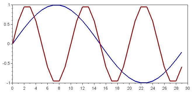
We’ll start by generating one-symbol sine waveforms at the binary 0 frequency (10 kHz) and the binary 1 frequency (30 kHz).

 

ZeroFrequency = 10e3;
OneFrequency = 30e3;
SamplingFrequency = 300e3;
Samples_per_Symbol = SamplingFrequency/ZeroFrequency;
n = 0:(Samples_per_Symbol-1);
Symbol_Zero = sin(2*%pi*n / (SamplingFrequency/ZeroFrequency));
Symbol_One = sin(2*%pi*n / (SamplingFrequency/OneFrequency));
plot(n, Symbol_Zero)
plot(n, Symbol_One)

 

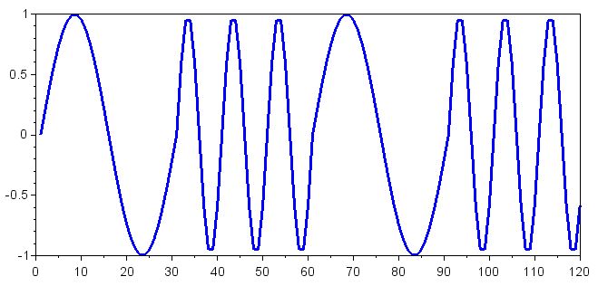
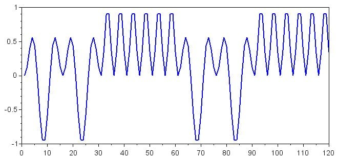
Now let’s create the received baseband signal. We can do this by concatenating Symbol_Zero and Symbol_One arrays; we’ll use the sequence 0101:

 

ReceivedSignal = [Symbol_Zero Symbol_One Symbol_Zero Symbol_One];
plot(ReceivedSignal)

 

Next, we multiply each symbol in the received signal by the waveform for a binary 0 symbol and by the waveform for a binary 1 symbol. We accomplish this step by concatenating Symbol_Zero and Symbol_One arrays according to the number of symbols in the received signal and then using element-wise multiplication; refer to this article for more information on element-wise multiplication in Scilab (or MATLAB).

 

Decoding_Zero = ReceivedSignal .* [Symbol_Zero Symbol_Zero Symbol_Zero Symbol_Zero];
Decoding_One = ReceivedSignal .* [Symbol_One Symbol_One Symbol_One Symbol_One];
plot(Decoding_Zero)

 

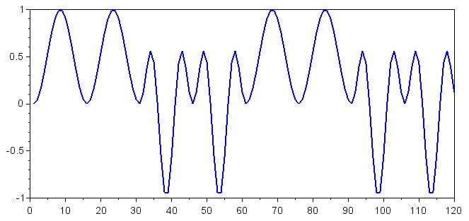
plot(Decoding_One)

 

Don’t be distracted by these rather complicated waveforms; all we’re interested in is the DC offset, which in mathematical terms is simply the mean. If we want to display the DC offset corresponding to each symbol, we first need to generate some new arrays:

 

for k=1:(length(Decoding_Zero)/Samples_per_Symbol)
  > SymbolOffsets_Zero(((k-1)*Samples_per_Symbol)+1:k*(Samples_per_Symbol)) = mean(Decoding_Zero(((k-1)*Samples_per_Symbol)+1:k*(Samples_per_Symbol)));
  > end


for k=1:(length(Decoding_One)/Samples_per_Symbol)
  > SymbolOffsets_One(((k-1)*Samples_per_Symbol)+1:k*(Samples_per_Symbol)) = mean(Decoding_One(((k-1)*Samples_per_Symbol)+1:k*(Samples_per_Symbol)));
  > end

 

You might need to ponder these commands a bit to understand exactly what I’m doing, but here’s the basic idea: The for loop is used to progress one symbol at a time through the Decoding_Zero and Decoding_One arrays. In the SymbolOffsets_Zero and SymbolOffsets_One arrays, all the data points corresponding to one symbol are filled with the mean of the relevant symbol in the Decoding_Zero and Decoding_One arrays. We have 30 samples per symbol, so the first command operates on array values 1 to 30, the next operates on array values 31 to 60, and so forth. Here are the results:

 

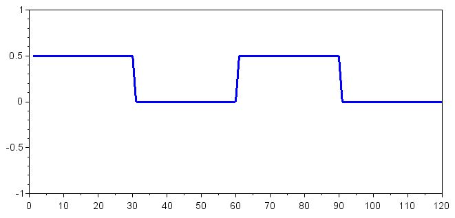
plot(SymbolOffsets_Zero)

 

plot(SymbolOffsets_One)

 

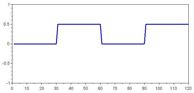
The SymbolOffsets_Zero array shows us the DC offset resulting from the multiplication of the received baseband symbol with the binary 0 frequency, and the SymbolOffsets_One array shows us the DC offset resulting from the multiplication of the received baseband symbol with the binary 1 frequency. We know that multiplying two similar frequencies will result in a relatively large DC offset. Thus, a value of 0.5 in the SymbolOffsets_Zero array indicates that the received symbol was a binary 0, and a value of 0.5 in the SymbolOffsets_One array indicates that the received symbol was a binary 1.

 

Conclusion

This article presented a mathematical approach for decoding FSK. The procedure was implemented in Scilab, but it would not be difficult to translate the Scilab commands into a high-level programming language such as C. We’ll continue working with FSK decoding in the next article.