How to Use Scilab to Analyze Amplitude-Modulated RF Signals

Scilab’s FFT functionality can help you understand the frequency-domain effects of RF modulation techniques.

Supporting Information

• Learning to Live in the Frequency Domain (from Chapter 1 of AAC’s RF textbook)
• The Many Types of Radio Frequency Modulation (and other pages in Chapter 4 of the RF textbook)

In a previous article, we introduced Scilab’s fft() command and discussed how we can manipulate FFT results so that they convey clear information about the amplitude of frequency components in a sampled signal. However, the FFT analysis performed in the previous article wasn’t particularly useful—it merely informed us that the sinusoid had one spectral component at a frequency that we specifically selected at the beginning of the procedure. This article should be more interesting: we’ll use discrete-time Fourier analysis to gain insight into the effects of amplitude modulation.

 

Modulation in the Frequency Domain

Modulation creates changes that are evident in a time-domain plot of the modulated signal. Why, then, do we need to generate a frequency-domain plot?

Well, for a full answer to that question I recommend the first textbook page listed in the Supporting Information section. The short answer is as follows: The spectrum of a modulated signal gives us an intuitive, clear representation of important information that is difficult—or in some cases virtually impossible—to extract from a time-domain plot. Spectral analysis can also help us to really understand what’s happening when we perform modulation; time-domain plots include details that are unnecessary when the goal is to ponder the fundamental interactions between the frequencies of the baseband signal and the frequency of the carrier signal.

 

Generating Frequency-Domain Plots for Modulated Signals

First, let’s set up our Scilab environment with variables that we will need throughout the rest of the article.

 

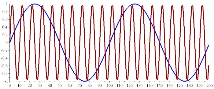
BasebandFrequency = 10e3;
CarrierFrequency = 100e3;
SamplingFrequency = 1e6;
BufferLength = 200;
n = 0:(BufferLength - 1);
BasebandSignal = sin(2*%pi*n / (SamplingFrequency/BasebandFrequency));
CarrierSignal = sin(2*%pi*n / (SamplingFrequency/CarrierFrequency));
plot(n, BasebandSignal)
plot(n, CarrierSignal)

Single-Frequency Amplitude Modulation

The basic mathematical relationship for amplitude modulation is as follows:

 

$$x_{AM}(t)=\sin(\omega_Ct)(1+x_{BB}(t))$$

 

The carrier is represented by the sin(ω_Ct) term, so what we’re doing here is shifting the baseband signal up (such that its values are always positive) and then multiplying the carrier by the shifted baseband. Here is the corresponding Scilab command:

 

ModulatedSignal_AM = CarrierSignal .* (1+BasebandSignal);

 

One very important detail is the period in front of the asterisk. In the Scilab environment, CarrierSignal and BasebandSignal are matrices, and if you use only an asterisk with two matrices, Scilab assumes that you want to perform matrix multiplication. In this situation we don’t want to perform matrix multiplication (and actually it’s not even possible, because the number of columns in the first matrix does not equal the number of rows in the second matrix).

We are trying to replicate typical analog multiplication, where the instantaneous value of one signal is repeatedly multiplied by the corresponding instantaneous value of another signal. This means that we need to use “element-wise” multiplication, where the first element in CarrierSignal is multiplied by the first element in BasebandSignal, the second element in CarrierSignal is multiplied by the second element in BasebandSignal, and so forth. We accomplish this by using the .* operator instead of the * operator.

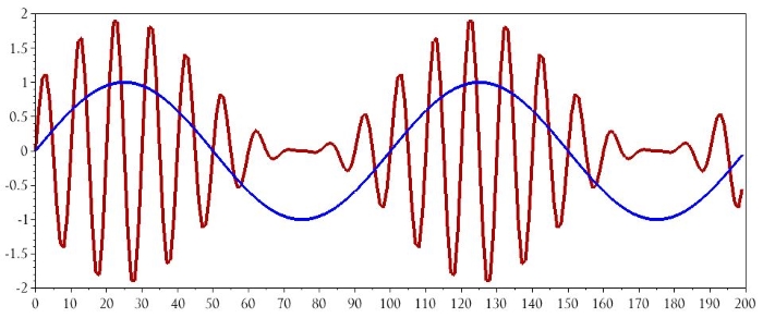
Here are the results in the time domain:

 

plot(n, BasebandSignal)
plot(n, ModulatedSignal_AM)

 

Now let’s set up our DFT horizontal axis:

 

HalfBufferLength = BufferLength/2;
HorizAxisIncrement = (SamplingFrequency/2)/HalfBufferLength;
DFTHorizAxis = 0:HorizAxisIncrement:((SamplingFrequency/2)-HorizAxisIncrement);

 

The following commands will produce the frequency-domain plot:

 

AM_DFT = fft(ModulatedSignal_AM);
AM_DFT_magnitude = abs(AM_DFT);
plot(DFTHorizAxis, AM_DFT_magnitude(1:HalfBufferLength))
xlabel("Frequency (Hz)")

 

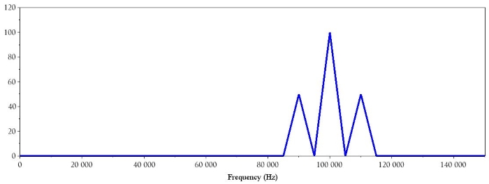
We have a spectrum consisting of a dominant spike at the carrier frequency and two sidebands corresponding to the carrier frequency plus the baseband frequency and the carrier frequency minus the baseband frequency. Multiplying the two signals has shifted the baseband spectrum (which has a spike at both positive 10 kHz and negative 10 kHz) such that it is centered on the carrier frequency.

Amplitude Modulation with Multiple Baseband Frequencies

Typically a baseband signal is not a single-frequency sinusoid—modulation is a way of transferring information using a higher-frequency carrier, and there isn’t much information to be found in an unchanging 10 kHz sine wave. If we transmit, say, a voice recording or a varying temperature measurement, the baseband signal’s frequency will vary within a certain range.

To produce a more realistic AM spectrum, we can create a baseband signal with multiple frequencies and then follow the same DFT procedure used above:

 

BufferLength = 1000;
n = 0:(BufferLength - 1);
Baseband_1 = sin(2*%pi*n / (SamplingFrequency/BasebandFrequency));
Baseband_2 = sin(2*%pi*n / (SamplingFrequency/(BasebandFrequency/2)));
Baseband_3 = sin(2*%pi*n / (SamplingFrequency/(BasebandFrequency/4)));
Baseband_4 = sin(2*%pi*n / (SamplingFrequency/(BasebandFrequency/8)));
Baseband_5 = sin(2*%pi*n / (SamplingFrequency/(BasebandFrequency/10)));
BasebandSignal = [Baseband_1 Baseband_2 Baseband_3 Baseband_4 Baseband_5];
BufferLength = BufferLength * 5;
n = 0:(BufferLength - 1);

 

What I did here is generate five sinusoids with different frequencies ranging from 1 kHz to 10 kHz (I increased the buffer length to 1000 so that each sinusoid would have at least one full cycle). I then concatenated these sinusoids into one long baseband signal (and I increased the buffer length accordingly). This is what the waveform looks like in the time domain:

 

 

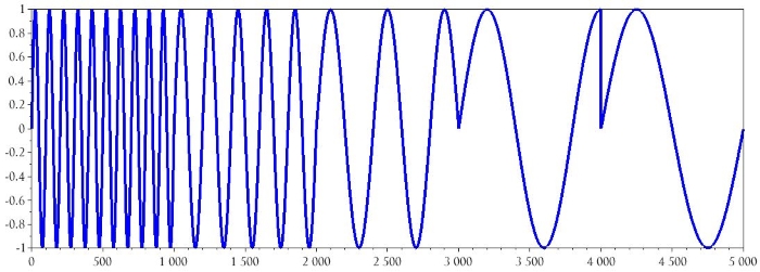
The frequency of the carrier doesn’t change, but we still need to generate a new waveform because the length of the CarrierSignal array has to be the same as the length of the BasebandSignal array.

 

CarrierSignal = sin(2*%pi*n / (SamplingFrequency/CarrierFrequency));

 

Now we generate a new amplitude-modulated signal, create a new series of values for the horizontal axis of the DFT, compute the FFT, and plot the data.

 

ModulatedSignal_AM = CarrierSignal .* (1+BasebandSignal);
HalfBufferLength = BufferLength/2;
HorizAxisIncrement = (SamplingFrequency/2)/HalfBufferLength;
DFTHorizAxis = 0:HorizAxisIncrement:((SamplingFrequency/2)-HorizAxisIncrement);
AM_DFT = fft(ModulatedSignal_AM);
AM_DFT_magnitude = abs(AM_DFT);
plot(DFTHorizAxis, AM_DFT_magnitude(1:HalfBufferLength))

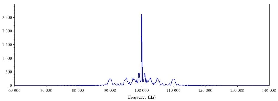
Click to enlarge.

 

Conclusion

In this article we used Scilab to investigate the frequency-domain effects of single-frequency amplitude modulation, and we also generated a variable-frequency baseband signal so that we could see an example of a more realistic AM spectrum. I plan to explore the spectral characteristics of frequency modulation in a future article.