Technical Article

Digital Signal Processing in Scilab: Understanding Phase Misalignment in FSK Decoding

September 28, 2018 by Robert Keim

In this article we’ll use Scilab to explore the effect of unpredictable phase variations in a demodulated frequency-shift-keying baseband signal.

In this article, we’ll use Scilab to explore the effect of unpredictable phase variations in a demodulated frequency-shift-keying baseband signal.

Related Information

Digital Modulation: Amplitude and Frequency (from Chapter 4 of AAC’s RF textbook)
How to Demodulate Digital Phase Modulation

Previous Articles on Scilab-Based Digital Signal Processing

In the previous article on how to decode an FSK signal, we saw that multiplication can be used to identify the frequency of a given portion of a received waveform. If we know that a symbol has one of two frequencies, we multiply the received signal by reference signals corresponding to the two frequencies, and the waveform resulting from this multiplication will have a relatively large DC offset if the frequency of the received symbol is similar to the frequency of the reference signal. This procedure is based on the following trig identity:

$$\sin(\omega_1t)*\sin(\omega_2t)=\frac{1}{2}(\cos((\omega_1-\omega_2)t)-\cos((\omega_1+\omega_2)t))$$

$$\cos(\omega_1t)*\cos(\omega_2t)=\frac{1}{2}(\cos((\omega_1-\omega_2)t)+\cos((\omega_1+\omega_2)t))$$

However, there’s an important detail here: these identities involve two sine waves or two cosine waves. In other words, the right side of the equation is valid only when the two multiplied waveforms have an aligned phase. What happens if the phase is not aligned? For example, what if the multiplied waveforms have a phase difference of 90°? Since sine and cosine are 90° out of phase, we can answer that question by examining another trig identity:

$$\sin(\omega_1t)*\cos(\omega_2t)=\frac{1}{2}(\sin((\omega_1+\omega_2)t)+\sin((\omega_1-\omega_2)t))$$

Now the situation is completely different. The right side of the equation has two sine terms instead of two cosine terms, and consequently, the relationship between input frequencies and DC offset is lost. If we input two waveforms of identical frequency and 90° phase difference, we have sin(0) instead of cos(0), and sin(0) = 0.

Generating and Visualizing Phase Differences

We can use a training sequence that precedes the actual packet to identify the point at which one symbol ends and the next symbol begins. In theory, this should allow us to establish transmitter-receiver synchronization that continues throughout the rest of the packet. This approach is not particularly robust, though, because phase shift in a received signal can occur rather quickly.

Multipath propagation contributes to phase shift, and conditions affecting multipath can change rapidly when the receiver, the transmitter, or nearby objects are in motion. Relative motion between the transmitter and the receiver also contributes to unpredictable phase variations. You may be able to establish phase alignment at the beginning of the packet, but this doesn’t mean that you’ll still have phase alignment toward the end of the packet or even in the middle of the packet.

We saw above that a 90° phase shift ruins the decoding algorithm. This represents the worst-case scenario; the performance of the decoding algorithm steadily diminishes as the phase difference between the received baseband signal and the reference signal approaches 90°.

Let’s look at some Scilab commands that will help us to visualize the effect of phase misalignment. First, we’ll create some variables and the two reference signals.

ZeroFrequency = 10e3;
OneFrequency = 30e3;
SamplingFrequency = 300e3;
Samples_per_Symbol = SamplingFrequency/ZeroFrequency;
n = 0:(Samples_per_Symbol-1);
Symbol_Zero = sin(2*%pi*n / (SamplingFrequency/ZeroFrequency));
Symbol_One = sin(2*%pi*n / (SamplingFrequency/OneFrequency));

Now we're going to generate a matrix that consists of eight received baseband signals with a phase that increases from 0° to 180° in increments of 22.5°.

for k = 0:8
  > Phase = k*(%pi/8);
  > RxSymbol = sin(Phase + (2*%pi*n / (SamplingFrequency/ZeroFrequency)));
  > RxSignal(k+1, 1:length(n)*4) = [RxSymbol RxSymbol RxSymbol RxSymbol];
  > end

To get to this point, we first create the RxSymbol array, which consists of one cycle, then we concatenate four of these symbols to create the baseband signal. The variable RxSignal is a multidimensional array—it contains 9 arrays, with each of these arrays being a series of values corresponding to a four-cycle baseband signal with a frequency of 10 kHz (i.e., the binary 0 frequency) and a phase of 0, 22.5°, 45°, 67.5°, 90°, 112.5°, 135°, 157.5°, or 180°.

The use of a multidimensional array makes it easy to generate a two-dimensional or three-dimensional plot of all the signals. A 2D plot can be generated as follows:

for k = 0:8
  > plot(RxSignal(k+1,😊)
  > end

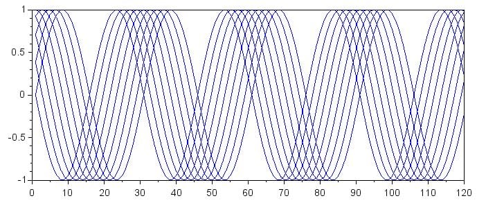
I prefer a 3D representation:

mesh(RxSignal)

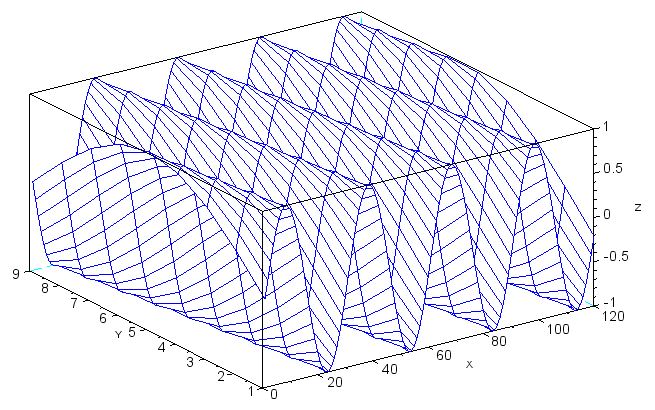
If you’re having trouble interpreting this plot, notice that the waveform at value 1 on the y-axis starts at a z-axis value of 0 and proceeds toward higher z-axis values. This is the sine wave with a phase term of zero. The starting point of the waveforms gradually changes as you move to higher numbers on the y-axis. Eventually, you reach value 9 on the y-axis, where the waveform starts at 0 but proceeds toward lower z-axis values; this is the sine wave with a phase shift of 180°.

The Effect of Phase Misalignment

We can now multiply all of these baseband signals by the binary 0 reference signal and then calculate the mean to see how the DC offset is affected by phase. Remember, all these signals have the same frequency; only the phase is changing.

for k = 0:8
  > Offsets_Zero(k+1, 1:length(n)*4) = mean(RxSignal(k+1, 😊 .* [Symbol_Zero Symbol_Zero Symbol_Zero Symbol_Zero]);
  > end
mesh(Offsets_Zero)

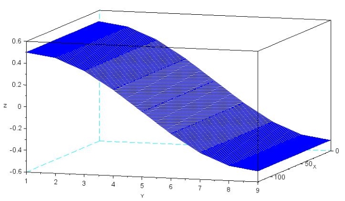
The following plot is more relevant to our discussion because we’re concerned with the magnitude of the offset, not the sign.

mesh(abs(Offsets_Zero))

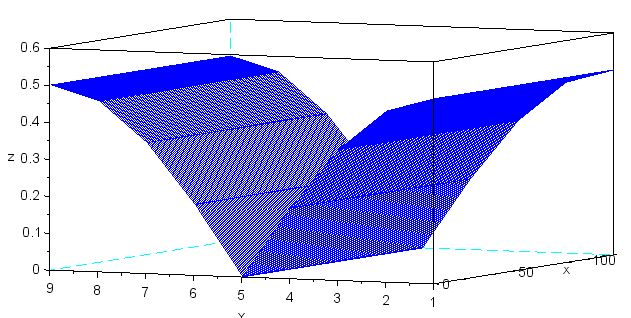
As you can see, the magnitude of the DC offset gradually decreases as the phase difference approaches 90°. Thus, if the phase difference between the received signal and the reference signal is close to 90°, the DC offset will indicate no significant similarity between the symbol frequency and the binary 0 frequency, even though the symbol frequency is exactly the same as the binary 0 frequency.

The Solution

The problem of phase misalignment can be overcome by incorporating quadrature demodulation into the receiver architecture.

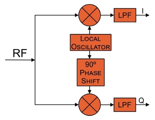
Quadrature demodulation produces two baseband signals that have a relative phase shift of 90°. These signals are referred to as I (in-phase) and Q (quadrature), and they are just what we need if we want to prevent the mathematical breakdown that occurs when the phase difference between the received symbol and the reference signal approaches 90°. The next article will explore the use of I/Q signals for improved FSK decoding.