How to Perform Frequency Modulation with a Digitized Audio Signal

In this article, we’ll use Scilab to create an FM waveform that carries information corresponding to an audio recording.

Supporting Information

• Learning to Live in the Frequency Domain (from Chapter 1 of AAC’s RF textbook)
• Frequency Modulation: Theory, Time Domain, Frequency Domain

Previous Articles on Scilab-Based Digital Signal Processing

• Introduction to Sinusoidal Signal Processing with Scilab
• How to Perform Frequency-Domain Analysis with Scilab
• How to Use Scilab to Analyze Amplitude-Modulated RF Signals
• How to Use Scilab to Analyze Frequency-Modulated RF Signals

In the previous article, we explored frequency modulation using a uniform, single-frequency sine wave as the baseband signal. This is a perfectly reasonable way to introduce the topic and gain familiarity with the basic concepts, but it’s not very practical. In most real-life applications, the baseband signal will be a complex waveform that exhibits changes in frequency and amplitude. These complex variations in frequency and amplitude are exactly what we find in audio signals, and as you know, frequency modulation is widely used to transmit sound information.

In this article, we’ll convert a sound file into a typical Scilab data array and then perform frequency modulation using this real-life data as the baseband signal. This should be a valuable exercise for those who are interested in software-defined radios. When we generate a digitized representation of an FM waveform, we’re creating a series of values that could be sent to a digital-to-analog converter, filtered, amplified, and transmitted. This allows you to implement a customized RF system without designing modulation circuitry.

Integrating a Baseband Signal

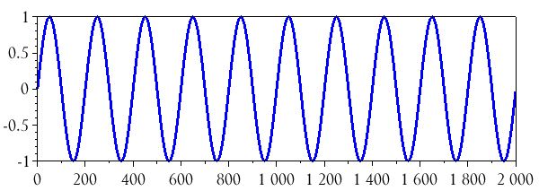
The Scilab command integrate() allows us to create a series of values corresponding to the indefinite integral of an existing series of values. (This is in contrast to a definite integral, which simply gives the area under the curve from a specified lower bound to a specified upper bound.) Let’s start with a basic sine wave:

BufferLength = 2000;
n = 0:(BufferLength - 1);
BasebandFrequency = 5e3;
SamplingFrequency = 1e6;
BasebandSignal = sin(2*%pi*n / (SamplingFrequency/BasebandFrequency));
plot(n, BasebandSignal)

The integrate() command needs four arguments. The first two are character strings (Scilab strings are enclosed in single or double quotation marks), the third is a number, and the fourth is a series of numbers.

• First argument: the function to be integrated, such as ‘f(x) = sin(x)’, but without the ‘f(x) =’ part.
• Second argument: the integration variable found in the expression given as the first argument, e.g., ‘x’.
• Third argument: the lower bound at which to start the integration procedure.
• Fourth argument: a series of values that establishes multiple upper bounds of integration.

For example:

BasebandSignal_integrated = integrate('sin(2*%pi*n / (SamplingFrequency/BasebandFrequency))', 'n', 0, n);
plot(n, BasebandSignal_integrated)

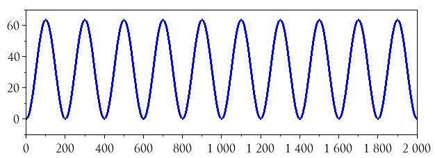
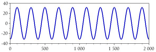
We know that the integral of a sine wave is a negative cosine wave (plus a constant), and the integrate() command did indeed produce a negative cosine wave, but it has a DC offset and the amplitude is not consistent with the amplitude of the original signal. These issues are easily corrected. First, we eliminate the DC offset by taking the average of the entire waveform and subtracting it from each value in the array:

BasebandSignal_integrated = BasebandSignal_integrated - mean(BasebandSignal_integrated);
plot(n, BasebandSignal_integrated)

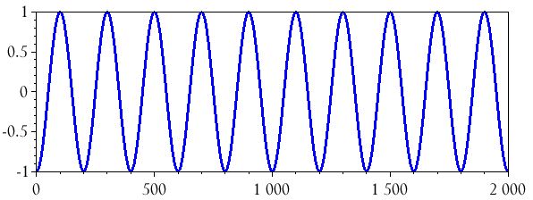
Next, we divide all the values in the array by the maximum value:

BasebandSignal_integrated = BasebandSignal_integrated ./ max(BasebandSignal_integrated);
plot(n, BasebandSignal_integrated)

Incorporating an Audio File

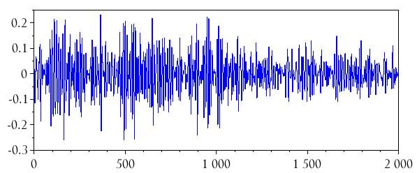
I downloaded an mp3 recording of a person saying the word “circuit,” then I converted it to a WAV file and loaded it into Scilab:

audio = wavread("C:\Users\Robert\Downloads\circuit.wav");

The resulting array had over 28,000 samples; I reduced it to a 2000-sample excerpt. I also transposed it (using the ' operator) so that it would have dimensions of 1×2000 instead of 2000×1:

audio = audio(11000:12999);
audio = audio';
plot(n, audio)

Integrating an Audio Signal

We’re going to use the inttrap() command to perform integration of our audio data. It appears that this procedure is mathematically equivalent to what we did above with the integrate() command; the reason I’m using inttrap() is that there is no way (as far as I can tell) to directly use integrate() with data that cannot be represented by an expression such as ‘sin(x)’.

The inttrap() command uses trapezoidal interpolation to calculate the definite integral (i.e., the area under the curve) of the waveform represented by an array of data. By repeatedly using inttrap() with a steadily increasing upper bound, we can produce a series of definite integrals that corresponds to the indefinite integral generated by integrate(); if you use this technique to generate an indefinite integral of a sine wave, you’ll see that the results are consistent with those obtained via integrate().

Here are the commands that I used to integrate the array audio:

for i=1:2000
  > audio_integrated(i) = inttrap(audio(1:i));
  > end

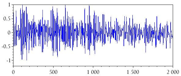
Now we’ll remove the DC offset (if the waveform has one) and scale the values into the range of approximately –1 to +1.

audio_integrated = audio_integrated - mean(audio_integrated);
audio_integrated = audio_integrated ./ max(audio_integrated);
plot(n, audio_integrated)

Changing the Sample Rate

There is one more thing we need to do before performing the modulation. In the previous article, we created the FM signal by generating a sine wave at the carrier frequency and including the integrated baseband signal as an added phase term. An important detail, though, is that we used a baseband sampling frequency that was high enough for the carrier-frequency signal. The WAV file that I used in this article has a sampling frequency of 44.1 kHz, which means that we can’t use the baseband sampling frequency for the modulation procedure—the sampling frequency must be at least twice the highest frequency in the modulated signal, and for a realistic system you probably want the sampling frequency to be at least five times the carrier frequency.

The next step, then, is to increase the sample rate of the integrated baseband signal. We can do this using the intdec() command. For example, let’s say the carrier frequency is 800 kHz and we decide to use a 4.41 MHz sampling frequency. This means that we will modify the audio_integrated array as follows:

SampleRate_IncreaseFactor = 4.41e6 / 44.1e3;
audio_integrated_upsampled = intdec(audio_integrated, SampleRate_IncreaseFactor);

The following two plots convey the results of the sample-rate modification.

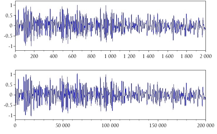
The waveforms look the same, and the horizontal axes show that the upsampled signal has 100 times more data points than the original signal.

Conclusion

At this point, we have an integrated audio baseband signal that is ready for the modulation command presented in the previous article. Overall I’m satisfied with the procedure that I’ve developed here, though I do wonder if there’s a better way to perform the integration. If you have any suggestions, feel free to share your thoughts in the comments section below.