 Facebook
 Google
 GitHub
 Linkedin
Frequency Modulation: Theory, Time Domain, Frequency Domain
We are all at least vaguely familiar with frequency modulation—it’s the origin of the term “FM radio.” If we think of frequency as something that has an instantaneous value, rather than as something that consists of several cycles divided by a corresponding period of time, we can continuously vary frequency in accordance with the instantaneous value of a baseband signal.
The Math
In the first page of this chapter, we discussed the paradoxical quantity referred to as instantaneous frequency. If you find this term unfamiliar or confusing, go back to that page and read through the “Frequency Modulation (FM) and Phase Modulation (PM)” section. You may still be a bit unsure, though, and that’s understandable—the idea of an instantaneous frequency violates the basic principle according to which “frequency” indicates how frequently a signal completes a full cycle: ten times per second, a million times per second, or whatever it may be.
We won’t attempt any sort of thorough or comprehensive treatment of instantaneous frequency as a mathematical concept. (If you’re determined to explore this issue in depth, here is an academic paper that should help.) In the context of FM, the important thing is to realize that instantaneous frequency follows naturally from the fact that the frequency of the carrier varies continuously in response to the modulating wave (i.e., the baseband signal). The instantaneous value of the baseband signal influences the frequency at a particular moment, not the frequency of one or more complete cycles.
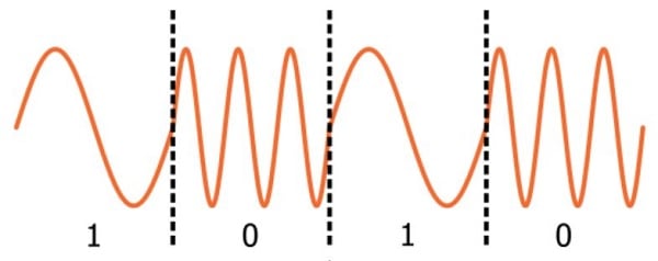
Actually, though, this is true only of analog FM; with digital FM, one bit corresponds to a discrete number of cycles. This leads to the interesting situation in which the older technology (analog FM) is less intuitive than the newer technology (digital FM, also called frequency shift keying, or FSK).
You don’t need to ponder instantaneous frequency in order to understand digital frequency modulation.
As in the previous page, we will write the carrier as sin(ωCt). It already has a frequency (namely, ωC), so we will use the term excess frequency to refer to the frequency component contributed by the modulation procedure. This term is slightly misleading, though, because “excess” implies a higher frequency, whereas modulation can result in a carrier frequency that is higher or lower than the nominal carrier frequency. In fact, this is why frequency modulation (in contrast to amplitude modulation) does not require a shifted baseband signal: Positive baseband values increase the carrier frequency and negative baseband values decrease the carrier frequency. Under these conditions demodulation is not a problem, because all baseband values map to a unique frequency.
Anyways, back to our carrier signal: sin(ωCt). If we add the baseband signal (xBB) to the quantity inside the parentheses, we are making the excess phase linearly proportional to the baseband signal. But we’re looking for frequency modulation, not phase modulation, so we want the excess frequency to be linearly proportional to the baseband signal. We know from the first page of this chapter that we can obtain frequency by taking the derivative, with respect to time, of phase. Thus, if we want the frequency to be proportional to xBB, we have to add not the baseband signal itself but rather the integral of the baseband signal (because taking the derivative cancels out the integral, and we are left with xBB as the excess frequency).
$$x_{FM}(t)=\sin(\omega_Ct+\int_{-\infty}^{t} x_{BB}(t)dt)$$
The only thing we need to add here is the modulation index, m. In the previous page we saw that the modulation index can be used to make the carrier’s amplitude variations more or less sensitive to the baseband-value variations. It’s function in FM is equivalent: the modulation index allows us to fine-tune the intensity of the change in frequency that is produced by a change in the baseband value.
$$x_{FM}(t)=\sin(\omega_Ct+m\int_{-\infty}^{t} x_{BB}(t)dt)$$
The Time Domain
Let’s look at some waveforms. Here is our 10 MHz carrier:
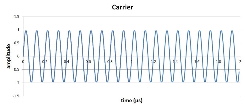
The baseband signal will be a 1 MHz sine wave, as follows:
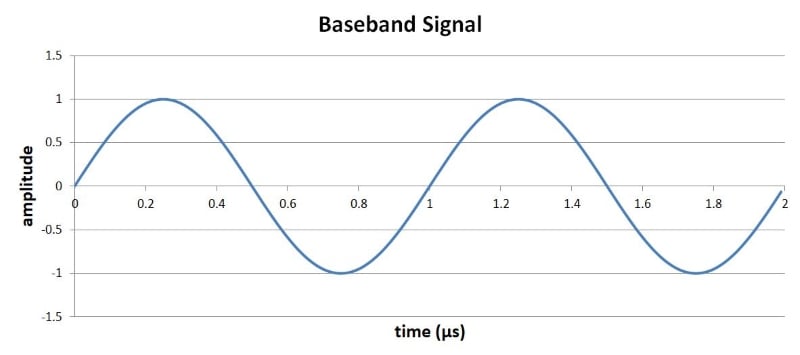
The FM waveform is generated by applying the formula given above. The integral of sin(x) is –cos(x) + C. The constant C is not relevant here, so we can use the following equation to compute the FM signal:
$$x_{FM}(t)=\sin((10\times10^6\times2\pi t)-\cos(1\times10^6\times2\pi t))$$
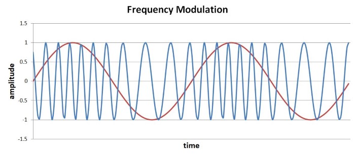
Here is the result (the baseband signal is shown in red):
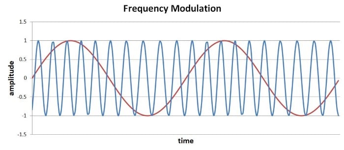
It almost seems that the carrier hasn’t changed, but if you look closely, the peaks are slightly closer together when the baseband signal is near its maximum value. So we do have frequency modulation here; the problem is that the baseband variations are not producing enough carrier-frequency variation. We can easily remedy this situation by increasing the modulation index. Let’s use m = 4:
$$x_{FM}(t)=\sin((10\times10^6\times2\pi t)-4\cos(1\times10^6\times2\pi t))$$
Now we can see more clearly how the frequency of the modulated carrier continuously tracks the instantaneous baseband value.
The Frequency Domain
AM and FM time-domain waveforms for the same baseband and carrier signals look very different. It is interesting, then, to find that AM and narrowband FM produce similar changes in the frequency domain. (Narrowband FM involves a limited modulating bandwidth and allows for easier analysis.) In both cases a low-frequency spectrum (including the negative frequencies) is translated to a band that extends above and below the carrier frequency. With AM, the baseband spectrum itself is shifted upwards. With FM, it is the spectrum of the integral of the baseband signal that appears in the band surrounding the carrier frequency.
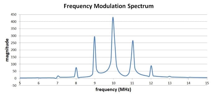
For the single-baseband-frequency, m-equals-1 modulation shown above, we have the following:
The next spectrum is with m = 4:
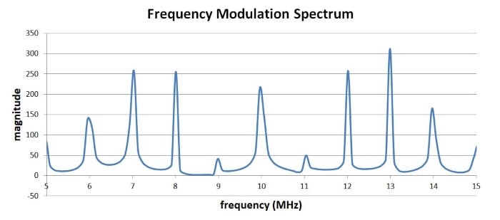
This demonstrates very clearly that the modulation index influences the frequency content of the modulated waveform. Spectral analysis with frequency modulation is more complicated than it is with amplitude modulation; it is difficult to predict the bandwidth of frequency-modulated signals.
Summary
- The mathematical representation of frequency modulation consists of a sinusoidal expression with the integral of the baseband signal added to the argument of the sine or cosine function.
- The modulation index can be used to make the frequency deviation more sensitive or less sensitive to variations in the baseband value.
- Narrowband frequency modulation results in a translation of the spectrum of the integral of the baseband signal to a band surrounding the carrier frequency.
- An FM spectrum is influenced by the modulation index as well as by the ratio of the amplitude of the modulating signal to the frequency of the modulating signal.


Shouldn’t the FM signal be
XFM(t)=sin((10×10^6×2πt)−(1/1×10^6×2π)cos(1×10^6×2πt))?