Facebook
 Google
 GitHub
 Linkedin
Amplitude Modulation in RF: Theory, Time Domain, Frequency Domain
We have seen that RF modulation is simply the intentional modification of the amplitude, frequency, or phase of a sinusoidal carrier signal. This modification is performed according to a specific scheme that is implemented by the transmitter and understood by the receiver. Amplitude modulation—which of course is the origin of the term “AM radio”—varies the amplitude of the carrier according to the instantaneous value of the baseband signal.
The Math
The mathematical relationship for amplitude modulation is simple and intuitive: you multiply the carrier by the baseband signal. The frequency of the carrier itself is not altered, but the amplitude will vary constantly according to the baseband value. (However, as we will see later, the amplitude variations introduce new frequency characteristics.) The one subtle detail here is the need to shift the baseband signal; we discussed this in the previous page. If we have a baseband waveform that varies between –1 and +1, the mathematical relationship can be expressed as follows:
$$x_{AM}=x_C(1+x_{BB})$$
where xAM is the amplitude-modulated waveform, xC is the carrier, and xBB is the baseband signal. We can take this a step further if we consider the carrier to be an endless, constant-amplitude, fixed-frequency sinusoid. If we assume that the carrier amplitude is 1, we can replace xC with sin(ωCt).
$$x_{AM}(t)=\sin(\omega_Ct)(1+x_{BB}(t))$$
So far so good, but there is one problem with this relationship: you have no control over the “intensity” of the modulation. In other words, the baseband-change-to-carrier-amplitude-change relationship is fixed. We cannot, for example, design the system such that a small change in the baseband value will create a large change in the carrier amplitude. To address this limitation, we introduce m, known as the modulation index.
$$ x_{AM}(t)=\sin(\omega_Ct)(1+mx_{BB}(t))$$
Now, by varying m we can control the intensity of the baseband signal’s effect on the carrier amplitude. Notice, however, that m is multiplied by the original baseband signal, not the shifted baseband. Thus, if xBB extends from –1 to +1, any value of m greater than 1 will cause (1 + mxBB) to extend into the negative portion of the y-axis—but this is exactly what we were trying to avoid by shifting it upwards in the first place. So remember, if a modulation index is used, the signal must be shifted based on the maximum amplitude of mxBB, not xBB.
The Time Domain
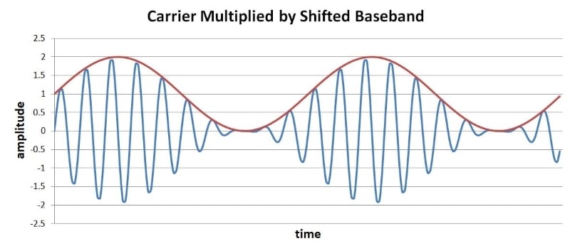
We looked at AM time-domain waveforms in the previous page. Here was the final plot (baseband in red, AM waveform in blue):
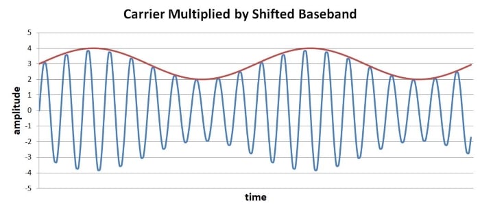
Now let’s look at the effect of the modulation index. Here is a similar plot, but this time I shifted the baseband signal by adding 3 instead of 1 (the original range is still –1 to +1).
Now we will incorporate a modulation index. The following plot is with m = 3.
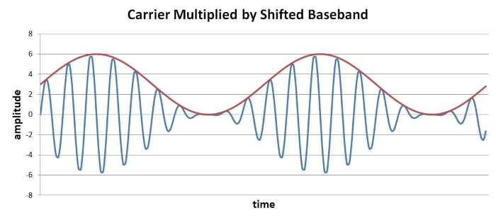
The carrier’s amplitude is now “more sensitive” to the varying value of the baseband signal. The shifted baseband does not enter the negative portion of the y-axis because I chose the DC offset according to the modulation index.
You might be wondering about something: How can we choose the correct DC offset without knowing the exact amplitude characteristics of the baseband signal? In other words, how can we ensure that the baseband waveform’s negative swing extends exactly to zero? Answer: You don’t need to. The previous two plots are equally valid AM waveforms; the baseband signal is faithfully transferred in both cases. Any DC offset that remains after demodulation is easily removed by a series capacitor. (The next chapter will cover demodulation.)
The Frequency Domain
As discussed in the second page of this textbook, RF development makes extensive use of frequency-domain analysis. We can inspect and evaluate a real-life modulated signal by measuring it with a spectrum analyzer, but this means that we need to know what the spectrum should look like.
Let’s start with the frequency-domain representation of a carrier signal:
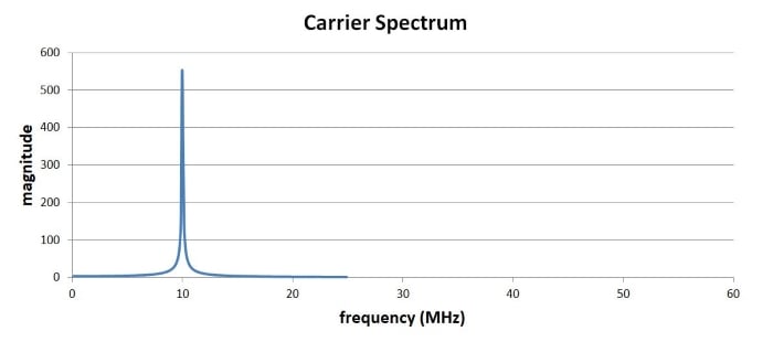
This is exactly what we expect for the unmodulated carrier: a single spike at 10 MHz. Now let’s look at the spectrum of a signal created by amplitude modulating the carrier with a constant-frequency 1 MHz sinusoid.
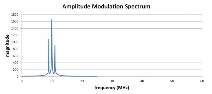
Here you see the standard characteristics of an amplitude-modulated waveform: the baseband signal has been shifted according to the frequency of the carrier. You could also think of this as “adding” the baseband frequencies onto the carrier signal, which is indeed what we’re doing when we use amplitude modulation—the carrier frequency remains, as you can see in the time-domain waveforms, but the amplitude variations constitute new frequency content that corresponds to the spectral characteristics of the baseband signal.
If we look more closely at the modulated spectrum, we can see that the two new peaks are 1 MHz (i.e., the baseband frequency) above and 1 MHz below the carrier frequency:
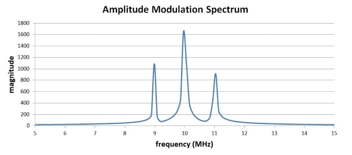
(In case you’re wondering, the asymmetry is an artifact of the calculation process; these plots were generated using real data, with limited resolution. An idealized spectrum would be symmetrical.)
Negative Frequencies
To summarize, then, amplitude modulation translates the baseband spectrum to a frequency band centered around the carrier frequency. There is something we need to explain, though: Why are there two peaks—one at the carrier frequency plus the baseband frequency, and another at the carrier frequency minus the baseband frequency? The answer becomes clear if we simply remember that a Fourier spectrum is symmetrical with respect to the y-axis; even though we often display only the positive frequencies, the negative portion of the x-axis contains corresponding negative frequencies. These negative frequencies are easily ignored when we’re dealing with the original spectrum, but it is essential to include the negative frequencies when we are shifting the spectrum.
The following diagram should clarify this situation.
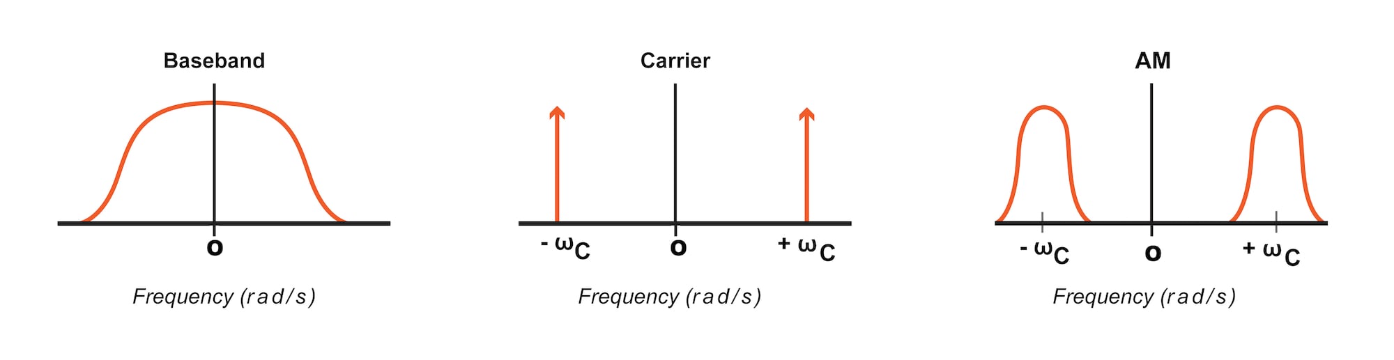
As you can see, the baseband spectrum and the carrier spectrum are symmetrical with respect to the y-axis. For the baseband signal, this results in a spectrum that extends continuously from the positive portion of the x-axis to the negative portion; for the carrier, we simply have two spikes, one at +ωC and one at –ωC. And the AM spectrum is, once again, symmetrical: the translated baseband spectrum appears in the positive portion and the negative portion of the x-axis.
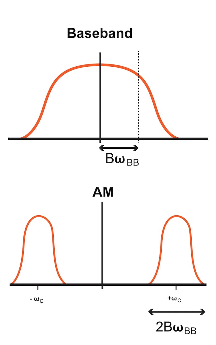
And here’s one more thing to keep in mind: amplitude modulation causes the bandwidth to increase by a factor of 2. We measure bandwidth using only the positive frequencies, so the baseband bandwidth is simply BWBB (see the diagram below). But after translating the entire spectrum (positive and negative frequencies), all the original frequencies become positive, such that the modulated bandwidth is 2BWBB.
Summary
- Amplitude modulation corresponds to multiplying the carrier by the shifted baseband signal.
- The modulation index can be used to make the carrier amplitude more (or less) sensitive to the variations in the value of the baseband signal.
- In the frequency domain, amplitude modulation corresponds to translating the baseband spectrum to a band surrounding the carrier frequency.
- Because the baseband spectrum is symmetrical with respect to the y-axis, this frequency translation results in a factor-of-2 increase in bandwidth.