 Facebook
 Google
 GitHub
 Linkedin
Digital Modulation: Amplitude and Frequency
Though far from extinct, analog modulation is simply incompatible with a digital world. We no longer focus our efforts on moving analog waveforms from one place to another. Rather, we want to move data: wireless networking, digitized audio signals, sensor measurements, and so forth. To transfer digital data, we use digital modulation.
We have to be careful, though, with this terminology. “Analog” and “digital” in this context refer to the type of information being transferred, not to the basic characteristics of the actual transmitted waveforms. Both analog and digital modulation use smoothly varying signals; the difference is that an analog-modulated signal is demodulated into an analog baseband waveform, whereas a digitally modulated signal consists of discrete modulation units, called symbols, that are interpreted as digital data.
There are analog and digital versions of the three modulation types. Let’s start with amplitude and frequency.
Digital Amplitude Modulation
This type of modulation is referred to as amplitude shift keying (ASK). The most basic case is “on-off keying” (OOK), and it corresponds almost directly to the mathematical relationship discussed in the page dedicated to [[analog amplitude modulation]]: If we use a digital signal as the baseband waveform, multiplying the baseband and the carrier results in a modulated waveform that is normal for logic high and “off” for logic low. The logic-high amplitude corresponds to the modulation index.
Time Domain
The following plot shows OOK generated using a 10 MHz carrier and a 1 MHz digital clock signal. We’re operating in the mathematical realm here, so the logic-high amplitude (and the carrier amplitude) is simply dimensionless “1”; in a real circuit you might have a 1 V carrier waveform and a 3.3 V logic signal.
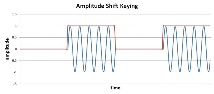
You may have noticed one inconsistency between this example and the mathematical relationship discussed in the [[Amplitude Modulation]] page: we didn’t shift the baseband signal. If you’re dealing with a typical DC-coupled digital waveform, no upward shifting is necessary because the signal remains in the positive portion of the y-axis.
Frequency Domain
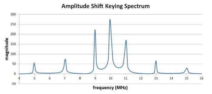
Here is the corresponding spectrum:
Compare this to the spectrum for amplitude modulation with a 1 MHz sine wave:
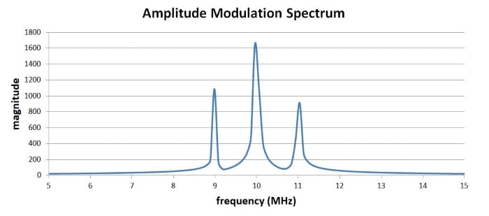
Most of the spectrum is the same—a spike at the carrier frequency (fC) and a spike at fC plus the baseband frequency and fC minus the baseband frequency. However, the ASK spectrum also has smaller spikes that correspond to the 3rd and 5th harmonics: The fundamental frequency (fF) is 1 MHz, which means that the 3rd harmonic (f3) is 3 MHz and the 5th harmonic (f5) is 5 MHz. So we have spikes at fC plus/minus fF, f3, and f5. And actually, if you were to expand the plot, you would see that the spikes continue according to this pattern.
This makes perfect sense. A Fourier transform of a square wave consists of a sine wave at the fundamental frequency along with decreasing-amplitude sine waves at the odd harmonics, and this harmonic content is what we see in the spectrum shown above.
This discussion leads us to an important practical point: abrupt transitions associated with digital modulation schemes produce (undesirable) higher-frequency content. We have to keep this in mind when we consider the actual bandwidth of the modulated signal and the presence of frequencies that could interfere with other devices.
Digital Frequency Modulation
This type of modulation is called frequency shift keying (FSK). For our purposes it is not necessary to consider a mathematical expression of FSK; rather, we can simply specify that we will have frequency f1 when the baseband data is logic 0 and frequency f2 when the baseband data is logic 1.
Time Domain
One method of generating the ready-for-transmission FSK waveform is to first create an analog baseband signal that switches between f1 and f2 according to the digital data. Here is an example of an FSK baseband waveform with f1 = 1 kHz and f2 = 3 kHz. To ensure that a symbol is the same duration for logic 0 and logic 1, we use one 1 kHz cycle and three 3 kHz cycles.
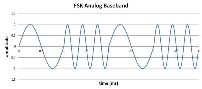
The baseband waveform is then shifted (using a mixer) up to the carrier frequency and transmitted. This approach is particularly handy in software-defined-radio systems: the analog baseband waveform is a low-frequency signal, and thus it can be generated mathematically then introduced into the analog realm by a DAC. Using a DAC to create the high-frequency transmitted signal would be much more difficult.
A more conceptually straightforward way to implement FSK is to simply have two carrier signals with different frequencies (f1 and f2); one or the other is routed to the output depending on the logic level of the binary data. This results in a final transmitted waveform that switches abruptly between two frequencies, much like the baseband FSK waveform above except that the difference between the two frequencies is much smaller in relation to the average frequency. In other words, if you were looking at a time-domain plot, it would be difficult to visually differentiate the f1 sections from the f2 sections because the difference between f1 and f2 is only a tiny fraction of f1 (or f2).
Frequency Domain
Let’s look at the effects of FSK in the frequency domain. We’ll use our same 10 MHz carrier frequency (or average carrier frequency in this case), and we’ll use ±1 MHz as the deviation. (This is unrealistic, but convenient for our current purposes.) So the transmitted signal will be 9 MHz for logic 0 and 11 MHz for logic 1. Here is the spectrum:
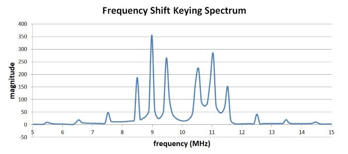
Note that there is no energy at the “carrier frequency.” This is not surprising, considering that the modulated signal is never at 10 MHz. It is always at either 10 MHz minus 1 MHz or 10 MHz plus 1 MHz, and this is precisely where we see the two dominant spikes: 9 MHz and 11 MHz.
But what about the other frequencies present in this spectrum? Well, FSK spectral analysis is not particularly straightforward. We know that there will be additional Fourier energy associated with the abrupt transitions between frequencies. It turns out that FSK results in a sinc-function type of spectrum for each frequency, i.e., one is centered on f1 and the other is centered on f2. These account for the additional frequency spikes seen on either side of the two dominant spikes.
Summary
- Digital amplitude modulation involves varying the amplitude of a carrier wave in discrete sections according to binary data.
- The most straightforward approach to digital amplitude modulation is on-off keying.
- With digital frequency modulation, the frequency of a carrier or a baseband signal is varied in discrete sections according to binary data.
- If we compare digital modulation to analog modulation, we see that the abrupt transitions created by digital modulation result in additional energy at frequencies farther from the carrier.


