Facebook
 Google
 GitHub
 Linkedin
Insight into the Results of DFT Analysis in Digital Signal Processing
This article attempts to give a deeper insight into the interpretation of DFT (direct Fourier transform) output.
A better insight into interpreting DFT (direct Fourier transform) analysis requires recognizing the consequences of two operations: the inevitable windowing when applying the DFT and the fact that the DFT gives only some samples of the signal's DTFT.
In the first part of this series, An Introduction to the Discrete Fourier Transform, we derived the N-point DFT equation for a finite-duration sequence, $$x(n)$$, as
$$X(k)=\sum\limits_{n=0}^{N-1}{x(n){{e}^{-j\tfrac{2\pi }{N}kn}}}$$
Equation 1
and the inverse DFT as
$$x(n)=\frac{1}{N}\sum\limits_{k=0}^{N-1}{X(k){{e}^{j\tfrac{2\pi }{N}kn}}}$$
Equation 2
We discussed an example which showed how the DFT helps us to represent a finite-duration sequence in terms of the complex exponentials. We saw that each of the DFT coefficients, $$X(k)$$, corresponds to a complex exponential at the normalized frequency of $$\frac{2\pi}{N}k$$.
This article will give more details about the interpretation of $$X(k)$$ in Equation 1. We will see that to get a better insight into interpreting the DFT output, we have to recognize the consequences of two operations: the inevitable windowing when applying the DFT and the fact that the DFT gives only some samples of the discrete-time Fourier transform (DTFT) of the finite-duration sequence.
At the end of the article, we will briefly review the DFT leakage phenomenon.
MATLAB Functions for the DFT Analysis
Before continuing, note that there are MATLAB functions which help us to avoid the tedious mathematics of Equations 1 and 2. These functions are fft(x) and ifft(X) which can, respectively, calculate Equations 1 and 2 in an efficient way. Let’s use these functions to find the DFT of $$x(n)$$ which was discussed in the previous article of this series. There, $$x(n)$$ was given as
| $$n$$ | $$0$$ | $$1$$ | $$2$$ | $$3$$ | $$4$$ | $$5$$ | $$6$$ | $$7$$ |
| $$x(n)$$ | $$0.2165$$ | $$0.8321$$ | $$0.7835$$ | $$0.5821$$ | $$0.2165$$ | $$-0.5821$$ | $$-1.2165$$ | $$-0.8321$$ |
To find the DFT coefficients, we can use this code:
x=[0.2165 0.8321 0.7835 0.5821 0.2165 -0.5821 -1.2165 -0.8321]
X=fft(x)
Then, we obtain X as given by the following table:
| $$k$$ | $$0$$ | $$1$$ | $$2$$ | $$3$$ | $$4$$ | $$5$$ | $$6$$ | $$7$$ |
| $$X(k)$$ | $$0$$ | $$-4j$$ | $$0.866-0.5j$$ | $$0$$ | $$0$$ | $$0$$ | $$0.866+0.5j$$ | $$4j$$ |
Now, using ifft(X), we can go back to the time domain and obtain $$x(n)$$ from these DFT coefficients.
The Inevitable Windowing When Applying the DFT
Assume that $$x(t)$$ is the continuous-time signal that we need to analyze and $$x'(n)$$ is the sequence obtained by sampling this continuous-time signal (see Figure 1 (a) and (b)).
Note that Figure 1 (b) shows the first eight samples in red to highlight that the DFT uses a windowed version of the input sequence.
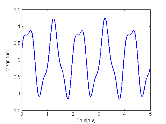
Figure 1 (a). The original continuous-time signal, $$x(t)$$, that we want to analyze.
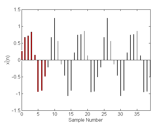
Figure 1 (b). $$x'(n)$$ which is the sampled version of the signal in Figure 1 (a).
Theoretically, $$x(t)$$ and $$x'(n)$$ can extend to positive and negative infinity on the time axis. However, to perform the N-point DFT, we can only use a finite-duration sequence such as $$x(n)$$ which is equal to $$x'(n)$$ only for $$n=0, 1, \dots, N-1$$. This is equivalent to multiplying $$x'(n)$$ by a rectangular window, $$w(n)$$, which is equal to one for $$n=0, 1, \dots, N-1$$ and zero otherwise.
Figure 1 (c) and (d) show the window function and $$x(n)$$ for $$N=8$$.
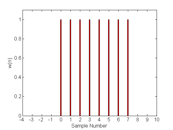
Figure 1 (c). The rectangular window function, $$w(n)$$, for $$N=8$$.
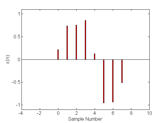
Figure 1 (d). The finite-duration sequence obtained by windowing $$x'(n)$$.
We should note that while we were originally looking for the spectrum of $$x(t)$$ through its samples $$x'(n)$$, we are in fact examining the windowed version of $$x'(n)$$ when applying the DFT. In other words, we will obtain the spectrum of the windowed signal instead of that of the original signal $$x'(n)$$.
The question is: How will this windowing operation alter the spectrum of the original signal?
Multiplication in the time domain is equivalent to convolution in the frequency domain, hence, the DTFT of the windowed signal will be
$$X\left( {{e}^{j\omega }} \right)=\frac{1}{2\pi }\int\limits_{2\pi }{{X}'\left( {{e}^{j\theta }} \right)}*W\left( {{e}^{j\left( \omega -\theta \right)}} \right)d\theta$$
Equation 3
where $$X'(e^{j\omega})$$ and $$W(e^{j\omega})$$ denote the DTFT of $$x'(n)$$ and $$w(n)$$, respectively. The above equation suggests that the spectrum of the windowed signal can be completely different from that of the original signal.
The reader can verify that the DTFT of $$w(n)$$ of length $$N$$ is given by
$$W({{e}^{j\omega }})={{e}^{-j\tfrac{\omega }{2}(N-1)}}\tfrac{Sin(N\tfrac{\omega }{2})}{Sin(\tfrac{\omega }{2})}$$
Equation 4
The magnitude of $$W(e^{j\omega})$$ for $$N=8$$ is shown in Figure 2. This figure shows an important property of the DTFT of $$w(n)$$: for $$\omega= \tfrac{2k\pi}{N}$$ and $$k$$ a nonzero integer, the magnitude of $$W(e^{j\omega})$$ is equal to zero and for $$k=0$$, we have $$W(e^{j\omega})=N$$. We will see how this property can result in misleading interpretation of the DFT analysis.
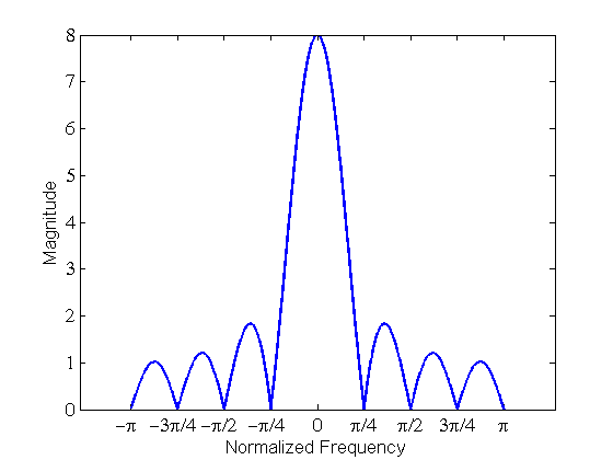
Figure 2. The magnitude of the spectrum of a rectangular window $$w(n)$$.
To clarify our discussion, let’s consider two simple examples. We apply the DFT to find the spectrum of $${{x}_{1}}\left( t \right)=Sin\left( 2\pi \times 1000^\text{ Hz}\times t \right)$$ and $${{x}_{2}}\left( t \right)=Sin\left( 2\pi \times 1500^\text{ Hz}\times t \right)$$. Assume that our sampling rate is $$8000$$ samples/second and we take eight samples of each of these two signals.
Example 1: The Eight-point DFT of $$x_{1}(n)$$
Sampling $$x_{1}(t)$$ leads to $$x_{1}'(n)$$. Applying the window function to $$x_{1}'(n)$$, we obtain $$x_{1}(n)$$ as
$${{x}_{1}}\left(n\right)={{x}_{1}}^{\prime}\left(n\right)w\left(n\right)$$
Equation 5
where $$x_1'(n)=sin(\tfrac{2n\pi}{8})$$. Using Euler's formula, we can rewrite Equation 5 as
$${{x}_{1}}(n)=\tfrac{{{e}^{j\tfrac{2n\pi }{8}}}-{{e}^{-j\tfrac{2n\pi }{8}}}}{2j}w\left( n \right)$$
Equation 6
Considering the frequency-shifting property of the DTFT, which gives the DTFT pair of $${{e}^{j{{\omega }_{0}}n}}x(n)\to X\left( {{e}^{j\left( \omega -{{\omega }_{0}} \right)}} \right)$$, we obtain
$${{X}_{1}}({{e}^{jw}})=\tfrac{1}{2j}\left( W\left( {{e}^{j\left( \omega -\tfrac{2\pi }{8} \right)}} \right)-W\left( {{e}^{j\left( \omega +\tfrac{2\pi }{8} \right)}} \right) \right)$$
Equation 7
Now, we can use Equation 4 with $$N=8$$ to plot the magnitude of the DTFT given by Equation 7. This is shown in Figure 3. This figure gives the spectrum of the windowed version of the original signal. While $$x_{1}'(n)$$ is the sum of two complex exponentials with frequencies of $$\tfrac{\pi}{4}$$ and $$-\tfrac{\pi}{4}$$, the spectrum of the windowed signal is a combination of two sinc-type functions given by Equation 4. The center of the sinc functions are shifted to $$\tfrac{\pi}{4}$$ and $$\tfrac{7\pi}{4}$$.
Note that, due to the periodic behavior of the discrete-time complex exponentials, the two frequencies $$-\tfrac{\pi}{4}$$ and $$\tfrac{7\pi}{4}$$ are the same. In other words, $$e^{j\tfrac{7\pi}{4}}=e^{-j\tfrac{\pi}{4}}$$.
In summary, while the input was a pure sinusoid, the spectrum of the windowed signal contains almost all frequency components.
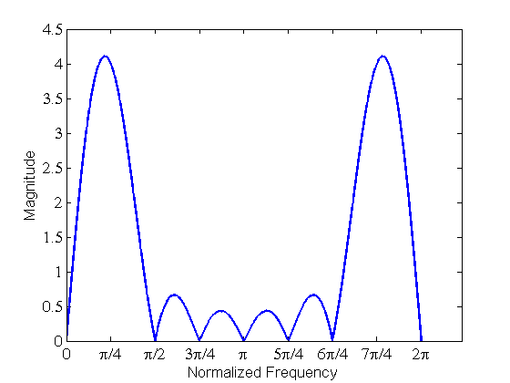
Figure 3. The magnitude of the spectrum given by Equation 7.
Based on the above discussion, we expect almost all frequency components to be present in a DFT analysis of sinusoidal signals. However, when the resolution of the DFT analysis is not sufficiently high, one may wrongly conclude that the finite-duration sequence consists of only a few frequency components.
For example, if we calculate the eight-point DFT of $$x_{1}(n)$$, we are looking at the values of the DTFT only at eight equally-spaced frequency points, i.e., at $$\omega=k\tfrac{2\pi}{8}$$ where $$k=0, 1, \dots, 7$$. Figure 4 compares the magnitude of the DFT outputs obtained by MATLAB’s fft(x) and $$X_{1}(e^{j\omega})$$ calculated by Equation 7. In this particular example, the frequency points of the DFT analysis are exactly at the frequencies that $$W(e^{j\omega})$$ becomes zero.
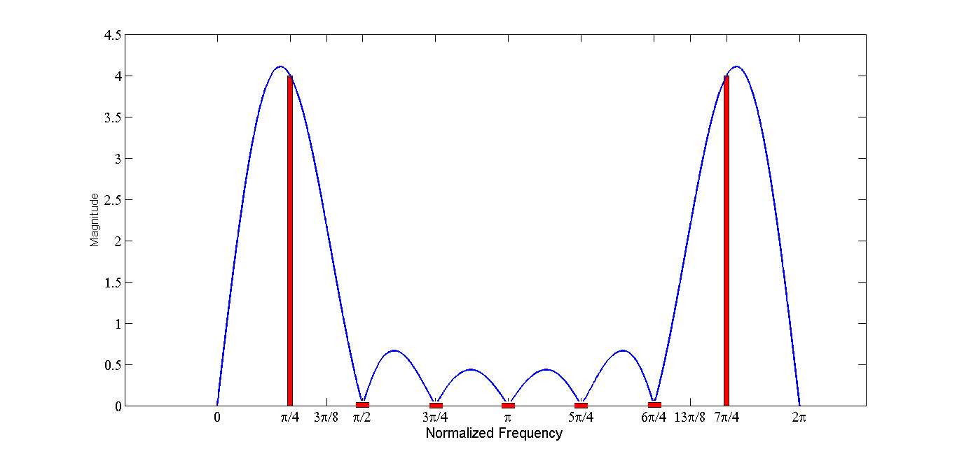
Figure 4. The magnitude of the DFT outputs (in red) and $$|X_{1}(e^{j\omega})|$$ calculated by Equation 7 (in blue).
Hence, based on this DFT analysis, one may wrongly conclude that $$x_{1}(n)$$ consists of only two frequency components at $$\tfrac{\pi}{4}$$ and $$\tfrac{7\pi}{4}$$. This is particularly misleading due to the fact that the original discrete-time signal $$x_{1}'(n)$$ was the sum of two complex exponentials at these frequencies.
However, we should remember that DFT gives only some samples of the DTFT and a windowed sinusoidal signal generally contains almost all frequency components. A technique called zero-padding can be used to find more frequency points for a given number of samples of $$x_{1}(t)$$. However, this article will not cover this technique due to the lack of space.
Example 2: The Eight-Point DFT of $$x_{2}(n)$$
The procedure to analyze $$x_{2}(n)$$ is similar to that of $$x_{1}(n)$$; however, $${{x}_{2}}^{\prime }\left( n \right)=Sin\left( \frac{3n\pi }{8} \right)$$ and Equation 7 will change to
$${{X}_{2}}({{e}^{j\omega}})=\tfrac{1}{2j}\left( W\left( {{e}^{j\left( \omega -\tfrac{3\pi }{8} \right)}} \right)-W\left( {{e}^{j\left( \omega +\tfrac{3\pi }{8} \right)}} \right) \right)$$
Equation 8
The magnitude of the DTFT and DFT of $$x_{2}(n)$$ are shown in Figure 5.

Figure 5. The magnitude of the DFT outputs (in red) and $$|X_{2}(e^{j\omega})|$$ calculated by Equation 8 (in blue).
In this figure, the center of the sinc functions are shifted to $$\frac{3\pi}{8}$$ and $$\frac{13\pi}{8}$$. Consequently, the zeros of the sinc-type functions do not coincide with the frequency points of the DFT. In fact, for a given N, the frequency points of the DFT is fixed and located at $$\frac{2\pi}{N}k$$, $$k=0, 1, \dots, N-1$$ regardless of the frequency of the input sequence; however, the center of the sinc functions is determined by the input frequency.
When the frequency of the input sequence exactly matches a DFT frequency point, zeros of the corresponding sinc function will coincide with the DFT frequencies. For example, the normalized frequency of $$x_{1}^{\prime}(n)$$ in the first example was $$\frac{\pi}{4}$$ which was equal to $$\frac{2\pi}{N}k$$ for $$N=8$$ and $$k=1$$.
A Brief Introduction to DFT Leakage
When we perform the DFT, we are calculating equally-spaced samples of the DTFT of the windowed signal. Hence, we are, in fact, analyzing the windowed signal.
From this point of view, the DFT obtained in Figure 4 is misleading because the DFT result suggests the presence of only two frequency components while the DTFT shows that the windowed signal contains many other frequency components. However, if we note that the original goal was to analyze the continuous-time signal, $$x(t)$$, through its samples, $$x^{\prime}(n)$$, rather than analyzing the windowed signal, we see that the DFT given by Figure 5 is misleading. This is because, in this case, the DFT cannot predict the frequency of the input sequence, $$x^{\prime}(n)$$, precisely.
While $$x^{\prime}(n)$$ can be written in terms of two components at $$\pm \frac{3\pi}{8}$$, the DFT result suggests presence of frequency components at $$\frac{2\pi}{8}k$$, $$k=0, 1, \dots, 7$$. This latter case, in which the frequency of the input sequence doesn’t exactly match a DFT frequency point, leads to DFT leakage. This means that the energy which was originally at frequencies $$\pm \frac{3\pi}{8}$$ is leaked to almost all other frequencies and we cannot predict the frequency components of the original signal successfully.
When we face DFT leakage, we can use different window types to mitigate the problem and estimate the frequency of the continuous-time signal more precisely. However, when performing the DFT analysis on real-world finite-length sequences, the DFT leakage is unavoidable.
Related Content