 Facebook
 Google
 GitHub
 Linkedin
An Introduction to the Discrete Fourier Transform
The DFT is one of the most powerful tools in digital signal processing which enables us to find the spectrum of a finite-duration signal.
The DFT is one of the most powerful tools in digital signal processing which enables us to find the spectrum of a finite-duration signal.
There are many circumstances in which we need to determine the frequency content of a time-domain signal. For example, we may have to analyze the spectrum of the output of an LC oscillator to see how much noise is present in the produced sine wave. This can be achieved by the discrete Fourier transform (DFT). The DFT is usually considered as one of the two most powerful tools in digital signal processing (the other one being digital filtering), and though we arrived at this topic introducing the problem of spectrum estimation, the DFT has several other applications in DSP.
Please note that this article tries to give a basic understanding of the DFT in an intuitive way; examining a list of its properties, as is usual in textbooks, is not the goal of this article.
Why the DFT?
Assume that $$x(t)$$, shown in Figure 1, is the continuous-time signal that we need to analyze.
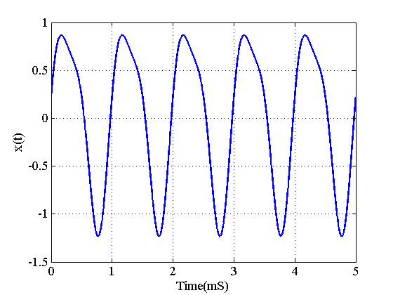
Figure 1. A continuous-time signal for which we need to determine the frequency content.
Obviously, a digital computer cannot work with a continuous-time signal and we need to take some samples of $$x(t)$$ and analyze these samples instead of the original signal. Moreover, while Figure 1 shows only the first $$5$$ millisecond of the signal, $$x(t)$$ may continue for hours, years, or more. Since our digital computer can process only a finite number of samples, we have to make an approximation and use a limited number of samples. Therefore, generally, a finite-duration sequence is utilized to represent this analog continuous-time signal which may extend to positive infinity on the time axis. The reader may wonder how many samples, $$L$$, we need in order to estimate the frequency content of a given signal. We will discuss this question in a future article of this series. For the time being, assume that we sample $$x(t)$$ in Figure 1 with a sampling rate of $$8000$$ samples/second and take only $$L=8$$ samples of this signal. The result is shown in red in Figure 2.
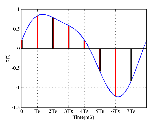
Figure 2. Sampling allows us to analyze continuous-time signals in a digital computer.
If we normalize the time axis to the sampling period $$T_s=\frac{1}{f_s}$$, we will obtain the discrete sequence $$x(n)$$, representing $$x(t)$$, as follows:
| $$n$$ | $$0$$ | $$1$$ | $$2$$ | $$3$$ | $$4$$ | $$5$$ | $$6$$ | $$7$$ |
| $$x(n)$$ | $$0.2165$$ | $$0.8321$$ | $$0.7835$$ | $$0.5821$$ | $$0.2165$$ | $$-0.5821$$ | $$-1.2165$$ | $$-0.8321$$ |
Fourier analysis provides several mathematical tools for determining the frequency content of a time-domain signal, but which tool is a good choice for analyzing $$x(n)$$? There are only two techniques from the Fourier analysis family which target discrete-time signals (see page 144 of this book): the discrete-time Fourier transform (DTFT) and the discrete Fourier transform (DFT).
The DTFT of an input sequence, $$x(n)$$, is given by
$$X(e^{j \omega})=\sum_{n=- \infty}^{+\infty}x(n)e^{-jn \omega}$$
Equation 1
The inverse of the DTFT is given by
$$x(n)=\frac{1}{2 \pi} \int_{- \pi}^{\pi} X(e^{j \omega})e^{jn \omega}d \omega$$
Equation 2
We can use Equation 1 to find the spectrum of a finite-duration signal $$x(n)$$; however, $$X(e^{j \omega})$$ given by the above equation is a continuous function of $$\omega$$. Hence, a digital computer cannot directly use Equation 1 to analyze $$x(n)$$. However, we can use samples of $$X(e^{j \omega})$$ to find an approximation of the spectrum of $$x(n)$$. The idea of sampling $$X(e^{j \omega})$$ at equally spaced frequency points is in fact the basis of the second Fourier technique mentioned above, i.e., the DFT. Note that this sampling is taking place in the frequency domain ($$X(e^{j \omega})$$ is a function of frequency ).
Performing the DFT Using Basic Math
Let’s proceed with the example started in the previous section. We have an L-sample-long sequence, $$x(n)$$, representing the analog continuous-time signal $$x(t)$$. The goal is to find a set of sinusoids which can be added together to produce $$x(n)$$.
As discussed above, the DFT is based on sampling the DTFT, given by Equation 1, at equally spaced frequency points. $$X(e^{j \omega})$$ is a periodic function in $$\omega$$ with a period of $$2 \pi$$. If we take $$N$$ samples in each period of $$X(e^{j \omega})$$, the spacing between frequency points will be $$\frac{ 2\pi }{N}$$. Hence, the frequency of the set of sinusoids that we are looking for will be of the form $$\frac{2 \pi}{N} \times k$$, where we can select $$k=0, 1, ..., N-1$$. Using complex exponentials similar to Equation 1 and 2, the basis functions will be $$e^{j \frac{2 \pi}{N}kn}$$. We are looking for a weighted sum of these functions which will hopefully give us the original signal $$x(n)$$. This means that
$$x(n)=\sum_{k=0}^{N-1}X'(k)e^{j\frac{2 \pi}{N}kn}$$ $$n=0, 1, \dots, L-1$$
Equation 3
where $$X'(k)$$ denotes the weight used for the complex exponential $$e^{j \frac{2 \pi}{N}kn}$$. Equation 3 is equivalent to the following set of equations
$$x(0)=X'(0)+X'(1)+X'(2)+ \dots +X'(N-1)$$
$$x(1)=X'(0)+X'(1)e^{j\frac{2 \pi}{N}}+X'(2)e^{j\frac{2\pi}{N}2}+ \dots +X'(N-1)e^{j\frac{2\pi}{N}(N-1)}$$
$$x(2)=X'(0)+X'(1)e^{j\frac{2\pi}{N}2}+X'(2)e^{j\frac{2\pi}{N}2\times 2}+ \dots +X'(N-1)e^{j\frac{2\pi}{N}(N-1)\times 2}$$
.
.
.
$$x(L-1)=X'(0)+X'(1)e^{j\frac{2\pi}{N}(L-1)}+X'(2)e^{j\frac{2\pi}{N}2\times(L-1)}+ \dots +X'(N-1)e^{j\frac{2\pi}{N}(N-1)\times(L-1)}$$
Equation 4
For a given $$L$$ and $$N$$, the values of complex exponentials are known and, having the value of the time-domain signal, we can calculate the coefficients $$X'(k)$$. The number of time-domain samples, $$L$$, gives the number of equations in the above set of equations, and the number of frequency-domain samples of $$X(e^{j\omega})$$ determines the number of unknowns in Equation 4. With $$L=N$$, there are $$N$$ linearly independent equations to find the $$N$$ unknowns, $$X'(k)$$.
Assuming $$L=N=8$$, we can find the matrix form of Equation 4 and use MATLAB to find the unknowns:
| $$k$$ | $$0$$ | $$1$$ | $$2$$ | $$3$$ | $$4$$ | $$5$$ | $$6$$ | $$7$$ |
| $$X'(k)$$ | $$0$$ | $$-0.5j$$ | $$0.1083-0.0625j$$ | $$0$$ | $$0$$ | $$0$$ | $$0.1083+0.0625j$$ | $$0.5j$$ |
What is the interpretation of this analysis? We decomposed the sequence $$x(n)$$ into a sum of complex exponentials given by Equation 3. Let’s substitute the results in the mentioned equation. With $$L=N=8$$ and omitting the exponentials with zero coefficients according to the above table, we obtain
$$x(n)=X'(1)e^{j\frac{2 \pi}{8}n}+X'(2)e^{j\frac{2\pi}{8}2n}+X'(6)e^{j\frac{2\pi}{8}6n}+X'(7)e^{j\frac{2\pi}{8}7n}$$
Since these exponential functions are periodic with $$N=8$$, we can further simplify this equation. For example, $$e^{j\frac{2\pi}{8}7n}$$ is equal to $$e^{j\frac{2\pi}{8}(8-1)n}=e^{j\frac{2\pi}{8}8n}e^{-j\frac{2\pi}{8}n}=e^{-j\frac{2\pi}{8}n}$$. After simplifying and rearranging the terms of the above equation, we have
$$x(n)=X'(1)e^{j\frac{2\pi}{8}n}+X'(7)e^{-j\frac{2\pi}{8}n}+X'(2)e^{j\frac{2\pi}{8}2n}+X'(6)e^{-j\frac{2\pi}{8}2n}$$
Finally, we obtain
$$x(n)=sin(\frac{2\pi}{8}n)+0.125sin(\frac{4\pi}{8}n)+0.2166cos(\frac{4\pi}{8}n)=sin(\frac{2\pi}{8}n)+0.25sin(\frac{4\pi}{8}n+3\frac{\pi}{3})$$
Equation 5
This shows that $$x(n)$$ can be represented by two components, one at the normalized frequency of $$\frac{2\pi}{8}$$ with an amplitude of $$1$$ and the other at $$\frac{4\pi}{8}$$ with an amplitude of $$0.25$$. These frequencies are normalized; if the sampling frequency is $$f_s=8000$$ samples/second, we obtain the frequency of these two components as $$f_1=\frac{2\pi}{8}\frac{f_s}{2\pi}=1 kHz$$ and $$f_2=\frac{4\pi}{8}\frac{f_s}{2\pi}=2 kHz$$.
Let’s summarize what we have discussed so far. We started with a continuous-time signal and used a finite number of samples to analyze the frequency content of this continuous-time signal. We saw that the problem of decomposing this discrete sequence boils down to solving a set of linear equations. In the case of this article’s simple example, we even simplified the result (Equation 5) and obtained an explicit equation for $$x(n)$$.
There is one point which needs further attention. The analysis started with a sequence of length eight which is shown in Figure 3. Clearly, we know the value of $$x(n)$$ for $$n=0, \dots, 7$$, but we don’t know $$x(n) $$ outside of this range. The above analysis is actually looking for a sum of complex exponentials which can reproduce the values of $$x(n)$$ for $$n=0, \dots, 7$$. Let’s examine Equation 5 outside of this range. To avoid ambiguity, we refer to the sequence given by Equation 5 as $$p(n)$$. $$p(n)$$, shown in Figure 4, is a periodic function with $$N=8$$. As shown in this figure, the values of the original $$x(n)$$ will be repeated every $$8$$ samples. In other words, while we could represent $$x(n)$$ using some complex exponentials, the obtained representation is periodic, and $$x(n)$$ is equal to $$p(n)$$ only in one period. When developing, discussing, and applying the DFT, always remember that we are achieving a representation of the finite-duration sequence using a periodic sequence, where the values in one period of this periodic sequence are equal to those in the finite-duration sequence.
Note that the periodic behaviour of $$p(n)$$ can also be understood by recalling that we are sampling $$X(e^{j\omega})$$, the DTFT of $$x(n)$$, in the frequency domain. In a previous article, we discussed how sampling a signal in the time domain leads to replicas of the origin signal in the frequency domain. We observe a similar phenomenon here: sampling $$X(e^{j\omega})$$ in the frequency domain leads to replicas of $$x(n)$$ in the time domain. The periodic form of $$x(n)$$ in Figure 3 is shown as $$p(n)$$ in Figure 4.
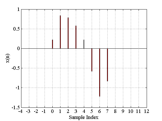
Figure 3. The analysis started using only these eight samples.
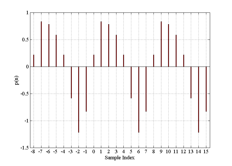
Figure 4. The analysis leads to p(n)which is the periodic form of x(n).
Deriving the DFT Equations
The discussed method for calculating the spectrum of a finite-duration sequence is simple and intuitive. It clarifies the inherent periodic behavior of DFT representation. However, it is possible to use the above discussion and derive closed-form DFT equations without the need to calculate the inverse of a large matrix. To this end, we only need to make a period signal out of the $$N$$ samples of the finite-duration sequence. Then, applying the discrete-time Fourier series expansion, we can find the frequency domain representation of the periodic signal. The obtained Fourier series coefficients are the same as the DFT coefficients except for a scaling factor.
Assume that the finite-duration sequence that we need to analyze is as shown in Figure 5 (a). To calculate the N-point DFT, we need to make a periodic signal, $$p(n)$$, from $$x(n)$$ with period $$N$$, as shown in Figure 5(b).
Considering the fact that $$p(n)=x(n)$$ for $$n=0, 1, \dots, N-1$$, we obtain the discrete-time Fourier series of this periodic signal
$$a_k=\frac{1}{N}\sum_{n=0}^{N-1}x(n)e^{-j\frac{2\pi}{N}kn}$$
Equation 6
where $$N$$ denotes the period of the signal. The time-domain signal can be obtained as follows:
$$x(n)=\sum_{k=0}^{N-1}a_{k}e^{j\frac{2\pi}{N}kn}$$
Equation 7
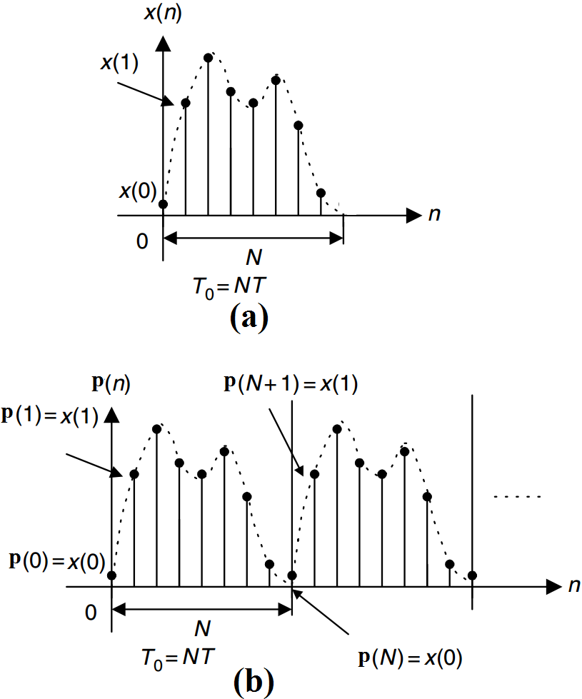
Figure 5. (a)The finite-duration sequence, x(n), to be analyzed. (b) The periodic signal obtained from x(n). Image courtesy of Digital Signal Processing, Fundamentals, and Applications.
Multiplying the coefficients given by Equation 6 by $$N$$, we obtain the DFT coefficients, $$X(k)$$, as follows:
$$X(k)=\sum_{n=0}^{N-1}x(n)e^{-j\frac{2\pi}{N}kn}$$
Equation 8
The inverse DFT will be
$$x(n)=\frac{1}{N}\sum_{k=0}^{N-1}X(k)e^{j\frac{2\pi}{N}kn}$$
Equation 9
Please note that while the discrete-time Fourier series of a signal is periodic, the DFT coefficients, $$X(k)$$, are a finite-duration sequence defined for $$0 \leq k \leq N-1$$.
Summary
- The DFT is one of the most powerful tools in digital signal processing; it enables us to find the spectrum of a finite-duration signal x(n).
- Basically, computing the DFT is equivalent to solving a set of linear equations.
- The DFT provides a representation of the finite-duration sequence using a periodic sequence, where one period of this periodic sequence is the same as the finite-duration sequence. As a result, we can use the discrete-time Fourier series to derive the DFT equations.
Related Content


I wonder how we can find the matrix form of Equation 4 and use MATLAB to find the coefficients?
Above Equation 5, the terms cancelled out. But what if the terms do not cancel out?
For example, if one term is with coefficient X’(4), then 8-4 = 4. There is no other terms to be paired with it, so how does it transform into another cos or sine wave?
Thank you