Facebook
 Google
 GitHub
 Linkedin
DFT Leakage and the Choice of the Window Function
This article will review the use of window functions to alleviate the DFT leakage.
This article will review the use of window functions to alleviate the DFT leakage.
In my last article, Insight into the Results of DFT Analysis in Digital Signal Processingrevious, we saw that it is possible to misinterpret the results of a Discrete Fourier Transform (DFT) analysis. The DFT leakage prevents us from precisely determining the frequency of the input sinusoid. This article will first examine the DFT leakage in more detail. Then it will explain how the use of different window functions can alleviate the problem.
DFT with No Leakage
Assume that, sampling at a rate of $$f_s$$, we obtain $$N$$ samples of the input sinusoid, $$x(t)=Asin(2\pi f_{in} \times t)$$, and, then, apply the N-point DFT to estimate the spectrum of the input signal. Based on our previous article, the spectrum of the windowed signal will be
$$X\left( e^{j\omega } \right)=\frac{A}{2j}\left( W\left( {{e}^{j(\omega-\frac{2\pi f_{in}}{f_{s}})}} \right)- W\left( {{e}^{j(\omega +\frac{2\pi f_{in}}{{{f}_{s}}})}} \right) \right)$$
Equation 1
where $$W(e^{j\omega})$$ denotes the spectrum of the rectangular window of length $$N$$ (see Equation 4 of this article). The N-point DFT will give the value of $$X(e^{j\omega})$$ at $$\omega=\tfrac{2\pi}{N}k$$, $$k=0, 1, \dots, N-1$$. Hence, we obtain the $$k$$th DFT value as
$$X\left( k \right)=\frac{A}{2j}\left( W\left( {{e}^{j(\frac{2\pi k}{N}-\frac{2\pi f_{in}}{f_s})}} \right)-W\left( {e^{j(\frac{2\pi k}{N}+\frac{2\pi {f_{in}}}{f_s})}} \right) \right)$$
Equation 2
Assume that the input frequency exactly matches a DFT frequency. In other words, there is an integer, $$k_1$$, that satisfies $$\tfrac{2\pi \times f_{in}} {f_s}=\tfrac{2\pi \times k_1}{N}$$, then we will have
$$X\left( k_1 \right)=\frac{A}{2j}\left( W\left( {{e}^{j(\frac{2\pi k_1}{N}-\frac{2\pi f_{in}}{f_s})}} \right)-W\left( {e^{j(\frac{2\pi k_1}{N}+\frac{2\pi {f_{in}}}{f_s})}} \right) \right)$$
Equation 3
This gives
$$X\left( {{k}_{1}} \right)=\frac{A}{2j}\left( W\left( {{e}^{j\times 0}} \right)-W\left( {{e}^{j\frac{2\pi {{k}_{1}}}{N}\times 2}} \right) \right)$$
Equation 4
We saw that the magnitude of the spectrum of a rectangular window, $$W(e^{j\omega})$$, is equal to zero for $$\omega=\tfrac{2\pi}{N}k$$ with $$k$$ a nonzero integer. However, for $$\omega=0$$, we have $$W(e^{j\omega})=N$$. Then Equation 4 gives
$$|X(k_{1})|=\frac{AN}{2}$$
Equation 5
This means that, without DFT leakage, a sinusoid with amplitude $$A$$ will lead to a DFT value of $$\tfrac{AN}{2}$$ in the corresponding frequency. For example, assume that $$x_{1}(t)=sin(2\pi \times1000^{\text{Hz}}\times t)$$, $$f_{s}=8000$$, and $$N=8$$, then we will obtain the value of the DFT equal to $$\tfrac{AN}{2}=\tfrac{1\times8}{2}=4$$ at the normalized frequency of $$f_{in}\times \tfrac{2\pi}{f_{s}}=1000 \times \tfrac{2\pi}{8000}=\tfrac{\pi}{4}$$.
In summary, when there is no DFT leakage, i.e., we can find $$k_{1}$$ in a way that $$\tfrac{2\pi \times f_{in}}{f_s}=\tfrac{2\pi k_{1}}{N}$$, we can determine the frequency content and the amplitude of each sinusoid present in the input signal. That’s why it is desirable to choose the parameters in a way that avoids the DFT leakage, but, in practice, this is not generally possible, and we can only alleviate the problem to some extent.
Remember that even if we had a combination of sinusoids at the input but the frequency of each of these sinusoids was a multiple of $$\tfrac{2\pi}{N}$$, then we could still use the results of this section to find the amplitude and frequency of different components of the input signal. For example, consider the eight-point DFT of $$x(n)$$ given by
$$x(n)=sin(\frac{2\pi}{8}n)+0.25sin(\frac{4\pi}{8}n+3)$$
Equation 6
Here, we have two sinusoids at normalized frequencies $$\tfrac{2\pi}{8}$$ and $$\tfrac{4\pi}{8}$$. With $$N=8$$, these two frequencies exactly match the DFT frequencies corresponding to $$X(1)$$ and $$X(2)$$. Hence, there is no DFT leakage and the DFT result can determine the frequency content and the amplitude of the components precisely. Based on the above discussion, we expect to find the DFT value of $$X(1)=\tfrac{AN}{2}=\tfrac{1 \times 8}{2}=4$$ and $$X(2)=\tfrac{AN}{2}=\tfrac{0.25 \times 8}{2}=1$$. An eight-sample long sequence obtained from Equation 6 is shown in Figure 1 and listed in the following table.
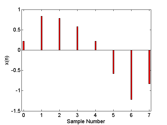
Figure 1. The eight-sample long sequence obtained from Equation 6.
| $$n$$ | $$0$$ | $$1$$ | $$2$$ | $$3$$ | $$4$$ | $$5$$ | $$6$$ | $$7$$ |
| $$x(n)$$ | $$0.2165$$ | $$0.8321$$ | $$0.7835$$ | $$0.5821$$ | $$0.2165$$ | $$-0.5821$$ | $$-1.2165$$ | $$-0.8321$$ |
Applying MATLAB’s fft(x) function to this sequence gives the DFT values as
| $$k$$ | $$0$$ | $$1$$ | $$2$$ | $$3$$ | $$4$$ | $$5$$ | $$6$$ | $$7$$ |
| $$X(k)$$ | $$0$$ | $$-4j$$ | $$0.866-0.5j$$ | $$0$$ | $$0$$ | $$0$$ | $$0.866+0.5j$$ | $$4j$$ |
which verifies the above discussion.
The Origin of the DFT Leakage
Equation 1 suggests that regardless of the input frequency, $$f_{in}$$, the discrete-time Fourier transform (DTFT) of the windowed sinusoid will be a combination of the shifted versions of the window spectrum $$W(e^{j\omega})$$. This clarifies the effect of the window spectrum on the value of the DFT that we will eventually obtain. For example, in the discussion of the previous section, we saw that, with no DFT leakage, a sinusoid with amplitude $$A$$ leads to a DFT value of $$\tfrac{AN}{2}$$ at the corresponding frequency. Here, $$N$$ arises from the fact that for a rectangular window of length $$N$$, we have $$W(e^{j\omega})=N$$ at $$\omega=0$$. In a similar manner, $$W(e^{j\omega})$$ affects the value of the DFT at frequencies other than $$\omega=0$$. We can think of the window function as a filter that alters the amplitude (and phase) of different components of the input signal.
With no DFT leakage, the particular shape of $$W(e^{j\omega})$$ is favourable and allows us to determine the input frequency precisely. However, when the input frequency does not exactly match a DFT frequency, we will not be able to precisely determine the frequency content of the input. To better envision this, see Figure 2 which illustrates the eight-point DFT of $$sin(\tfrac{3n\pi}{8})$$. The figure shows DTFT of the input sequence with the continuous curve in blue and the corresponding DFT with bars in red. In this example, the normalized input frequency is $$\tfrac{3\pi}{8}$$ which is not a multiple of $$\tfrac{2\pi}{N}=\tfrac{2\pi}{8}$$ and, hence, we expect the DFT leakage. The two frequencies $$\tfrac{\pi}{4}$$ and $$\tfrac{\pi}{2}$$ are the closest DFT frequencies to the input frequency and it is reasonable to see the largest DFT values at these two frequencies. However, we observe relatively strong components at $$\tfrac{3\pi}{4}$$, $$\pi$$, and $$\tfrac{5\pi}{4}$$ only because the magnitude response of the window function cannot abruptly roll-off. If we could reduce $$W(e^{j\omega})$$ more abruptly, we could reduce the leakage to these frequencies.

Figure 2. The DTFT (in blue) and the eight-point DFT (in red) of $$sin(\tfrac{3n\pi}{8})$$.
In summary, the magnitude of the window spectrum determines how much DFT leakage we will experience and if we can abruptly reduce the magnitude of $$W(e^{j\omega})$$ for $$\omega \neq 0$$, the leakage will be less severe. This brings us to the idea that maybe we can find another window function which exhibits a more abrupt roll-off in the magnitude response. In fact, though windowing is inevitable when performing the DFT, we will see that there are window functions with a much better performance than that of a rectangular function.
Other Window Function
The spectrum of a rectangular window normalized to the window length, $$\tfrac{W(e^{j\omega})}{N}$$, for $$N=8$$, is shown in Figure 3. The figure also illustrates the important parameters of a window function, i.e., the peak sidelobe (PSL) and the mainlobe width. The main lobe width can be calculated by subtracting the first two roots of $$W(e^{j\omega})$$ which, based on Equation 4 of this article, will be $$\tfrac{4\pi}{N}$$ for a rectangular window of length $$N$$. The peak sidelobe of a window is defined as the amplitude of the largest sidelobe relative to the amplitude of the mainlobe and is usually expressed in dB. For a rectangular window, we obtain $$PSL=20log(0.22) \approx -13$$dB.
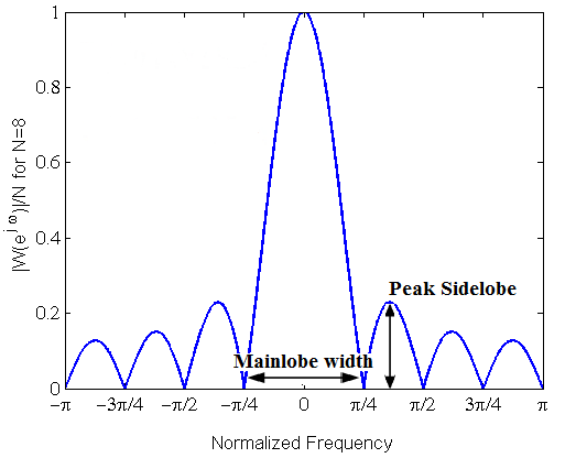
Figure 3.The spectrum of a rectangular window normalized to the window length for $$N=8$$.
To reduce the DFT leakage, we desire to decrease both the mainlobe width and the peak sidelobe. Since the mainlobe width of a rectangular window is $$\tfrac{4\pi}{N}$$, we can increase the number of samples to reduce the mainlobe width. However, the PSL of a rectangular window is almost independent of $$N$$. Hence, we have to use other types of windows to have a smaller PSL.
Table 1 lists some of the most popular window functions and their properties. The normalized Fourier transform of these window functions for $$N=21$$ is illustrated in Figure 4. Table 1 shows that, with a fixed window length, there is a trade-off between the main lobe width and the PSL and as we reduce the peak sidelobe, the width of the mainlobe increases. Note that, although Table 1 gives the approximate mainlobe width of the Bartlett, Hann, and Hamming equal to $$\tfrac{8\pi}{N}$$, the mainlobe width of these windows are not exactly the same and the mentioned trade-off is observed for these three windows too (see Figure 3).
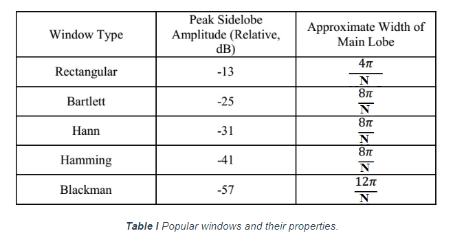
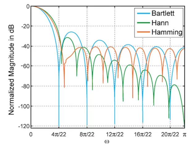
Figure 4. The normalized Fourier transform of the Bartlett, Hann, and Hamming windows for $$N=21$$.
A Suitable Window Reduces the DFT Leakage
Now, let’s see an example of how the choice of the window function allows us to estimate the frequency content of a signal more precisely. Assume that we want to analyze $$x(t)=sin(2\pi \times 1300^{\text{Hz}} \times t)+0.05sin(2\pi \times1950^{\text{Hz}} \times t)$$. In this case, we have a strong signal accompanying a weak one and the DFT leakage of the strong component may make it difficult to predict the presence of the weak component. Suppose that we take $$128$$ samples with a sampling rate of $$8000$$ samples/second. The normalized input frequencies of the two components of the input are $$1300 \times \tfrac{2\pi}{8000}=\tfrac{13\pi}{40}$$ and $$1950 \times \tfrac{2\pi}{8000}=\tfrac{39\pi}{80}$$. These frequencies are not a multiple of $$\tfrac{2\pi}{N}=\tfrac{2\pi}{128}$$ and we expect the DFT leakage. Figure 5 shows the 128-point DFT of $$x(t)$$. As shown in this figure, the large sidelobes of the rectangular window makes it difficult to detect the weak component of $$x(t)$$ because it is only slightly higher than the DFT values around $$1950$$ Hz. Note that the horizontal axis of this figure spans from DC to $$\tfrac{f_s}{2}=4000$$ Hz.

Figure 5. The 128-point DFT of $$x(t)$$ using a rectangular window.
To reduce the DFT leakage, we repeat the same analysis with a Hann window of length $$128$$. The result of this analysis is shown in Figure 6.

Figure 6. The 128-point DFT of $$x(t)$$ using a Hann window.
The DFT leakage still does not allow us to determine the frequency components of the input accurately. However, the utilized window gives us a more precise image of the frequency content of the input. For example, unlike Figure 5, Figure 6 predicts that there is no strong component neither from $$1600$$ to $$1800$$ Hz nor below $$1000$$Hz.
Summary
- Without the DFT leakage, a sinusoid with amplitude $$A$$ will lead to a DFT value of $$\tfrac{AN}{2}$$ in the corresponding frequency.
- The magnitude of the window spectrum determines how much DFT leakage we will experience and if we can abruptly reduce the magnitude of $$W(e^{j\omega})$$ for $$\omega \neq 0$$, the leakage will be less severe.
- To reduce the DFT leakage, we desire to decrease both the mainlobe width and the peak sidelobe of the window function.
- When we have a strong signal accompanying a weak one, the DFT leakage of the strong component may make it difficult to predict the presence of the weak component. However, the use of different window functions helps us to obtain a more precise image of the frequency content of the input.
Related Content