Analyzing a First-Order PLL in Acquisition Mode With a Nonlinear Model

In the previous article, we created a nonlinear model for analog PLLs. Here, we will apply the nonlinear model to a first-order PLL. We'll start by using it to characterize the PLL's dynamic behavior as it tries to lock onto the input. Then, by linearizing the nonlinear model, we'll analyze the effect of different loop parameters on the PLL's operation in the locked condition.

 

Nonlinear Model of a PLL

Shown in Figure 1 is the basic block diagram of a PLL with a multiplier phase detector.

 

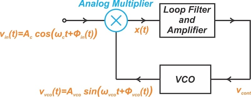
Figure 1. Basic block diagram of a PLL.

 

The nonlinear model of this system is shown in Figure 2.

 

Figure 2. Nonlinear model of a PLL with a multiplier phase detector.

 

In the above figure, ϕ_in is the input phase and ϕ_vco is the output phase. The phase error (ϕ_e) is defined as:

$$\phi_{e}(t) ~=~ \phi_{in}(t) ~-~ \phi_{vco}(t)$$

Equation 1.

 

Deriving the PLL's Integro-Differential Equation

We now try to express the phase error (ϕ_e) in terms of the input phase (ϕ_in). Assuming that input and the VCO are at the same frequency (ω_c = ω_vco), the signal at the output of the phase detector is:

$$x(t) ~=~ \frac{A_{c} A_{vco}k_d}{2} \sin \Big [ \phi_{in}(t)~-~ \phi_{vco}(t) \Big ] ~=~ \frac{A_{c} A_{vco}k_d}{2} \sin \big (\phi_{e}(t) \big )$$

Equation 2.

 

where k_d is the multiplicative factor associated with the phase detector.

The loop filter operates on x(t) to produce the VCO's control voltage (v_cont), which can be obtained by the following convolution integral:

$$v_{cont}(t) ~=~ \int_{-\infty}^{+\infty} x(\tau)h(t~-~\tau) d\tau$$

Equation 3.

 

where h(t) is the impulse response of the loop filter.

To proceed with our analysis of the feedback loop, we need to relate v_cont to the VCO's output phase. If ϕ_vco denotes the VCO's excess phase, we have:

$$\phi_{vco}(t) ~=~ k_{vco} \int_0^{t} v_{cont}(t) \ dt$$

Equation 4.

 

where k_vco is the frequency sensitivity.

We can take the derivative of the above equation to obtain the following relationship:

$$\frac{d}{dt}\phi_{vco}(t) ~=~ k_{vco} v_{cont}(t)$$

Equation 5.

 

The above equations describe the input-output characteristics of the various blocks within the feedback loop. We now combine these equations to relate ϕ_in to the VCO's output phase (ϕ_vco). Taking the derivative of Equation 1 and applying Equation 5, we obtain:

$$\frac{d}{dt}\phi_{vco}(t) ~=~ k_{vco} v_{cont}(t)$$

Equation 6.

 

Note that ϕ_e, ϕ_in, and v_cont are all functions of t, but we are omitting the dependence for the sake of notational simplicity. Substituting v_cont from Equation 3 into Equation 6 yields:

$$\frac{d \phi_{e}}{dt} ~=~ \frac{d \phi_{in}}{dt} ~-~ k_{vco} ~\times~ \int_{-\infty}^{+\infty} ~x~(\tau)h(t~-~\tau) d\tau$$

Equation 7.

 

Finally, we substitute for x(t) from Equation 2, producing:

$$\frac{d \phi_{e}}{dt} =~~ \frac{d \phi_{in}}{dt} ~-~ K_{0} ~\times~ \int_{-\infty}^{+\infty} \sin \big (\phi_{e}(\tau) \big ) h(t~-~\tau) d\tau$$

Equation 8.

 

where K₀, the loop gain, is described by the following equation:

$$K_0~=~ \frac{1}{2}A_cA_{vco}k_dk_{vco}$$

Equation 9.

 

In the above equation, both A_c and A_vco are measured in volts. The multiplicative factor associated with the phase detector (k_d) is measured in inverse volts (1/V). The frequency sensitivity (k_vco) is in radians per second per volt (rad/sV). K₀ is therefore expressed in terms of radians per second (rad/s).

 

The First-Order PLL

Let's apply our analysis to the simple case of a first-order PLL where the loop filter's transfer function is H(s) = 1 in the frequency domain. In this case, no loop filtering is included. We therefore obtain the block diagram shown in Figure 3.

 

Figure 3. Nonlinear model of a first-order PLL with a multiplier phase detector.

 

Noting that v_cont = x(t), we can combine Equations 2 and 6 to obtain:

$$\frac{d \phi_{e}}{dt} ~=~ \frac{d \phi_{in}}{dt} ~-~ \underbrace{\frac{1}{2}A_{c}A_{vco}k_{d}k_{vco}}_{K_0} ~\times~ \sin (\phi_{e} )$$

Equation 10.

 

The same result can be obtained from the general expression shown in Equation 8. For a filter with transfer function H(s) = 1, the impulse response h(t) is given by:

$$h(t)~=~\delta (t)$$

Equation 11.

 

where δ(t) is the Dirac delta function. Using the sifting property of the Dirac delta function, we can simplify the integral in Equation 8, producing:

$$\frac{d \phi_{e}}{dt} ~=~ \frac{d \phi_{in}}{dt} ~-~ K_{0} ~\times~ \sin (\phi_{e} )$$

Equation 12.

 

Although an analytical solution for Equation 12 isn't possible, we can solve it using numerical methods. Interestingly, even without solving this nonlinear differential equation, we can use it to gain insight into the behavior of a first-order PLL operating in the acquisition mode.

 

What is the Sifting Property?

The sifting property of the Dirac delta function states that for any continuous function f(t), the integral of f(t) multiplied by the Dirac delta function δ(t – t₀) over the entire real line is equal to the value of f(t) at t = t₀.

 

Acquisition Mode of a First-Order PLL

Let's consider the problem of frequency and phase acquisition for the PLL. Assume that the PLL input is:

$$v_{in} ~=~ A_c \ \cos(\omega_c t~+~ \phi_1)$$

Equation 13.

 

and the VCO output is:

$$v_{vco} ~=~ A_{vco} \cos(\omega_{vco} t~+~ \phi_{vco})$$

Equation 14.

 

The input and the VCO are not at the same frequency. To apply the analysis we provided earlier in the article, we can express the input signal as:

$$v_{in} ~=~ A_c \ \cos \big( \omega_{vco} t~+~ \underbrace{(\omega_c ~-~ \omega_{vco}) t ~+~ \phi_1}_{\phi_{in}} \big )$$

Equation 15.

 

Therefore, in this case, the input phase is:

$$\phi_{in} ~=~ (\omega_c ~-~ \omega_{vco}) t ~+~ \phi_1$$

Equation 16.

 

We find the time derivative of the input phase and substitute the result into Equation 12:

$$\frac{d \phi_{e}}{dt} ~=~ \underbrace{(\omega_c ~-~ \omega_{vco})}_{\Delta \omega} ~-~ K_{0} ~\times~ \sin (\phi_{e} )$$

Equation 17.

 

where Δ⍵ is the frequency step applied to the PLL input.

Using the above equation, we can plot the time derivative of the phase error (dϕ_e/dt) as a function of the phase error (ϕ_e). The result is what's known in the PLL literature as a phase-plane plot.

Figure 4 shows the typical phase-plane plot of a first-order PLL. As we'll discuss shortly, this plot is obtained when Δ⍵ < K₀.

 

Figure 4. Phase-plane showing the trajectory of a first-order PLL.

 

This plot provides useful insights into the PLL operation. Three observations in particular come to mind here.

First, the phase-plane plot for a first-order PLL is a vertically shifted sinusoid. Since –1 ≤ sin(ϕ_e) ≤ 1, the maximum and minimum of dϕ_e/dt are Δ⍵ + K₀ and Δ⍵ – K₀, respectively. Additionally, at ϕ_e = 0, we have dϕ_e/dt = Δ⍵.

Second, the PLL follows the trajectory of this plot as it tries to lock onto the input signal and track it.

Third, the points where dϕ_e/dt equals zero are the points at which the system is at equilibrium. To understand this, note that dϕ_e/dt = 0 implies that the phase error (ϕ_e) is constant. A constant ϕ_e produces a constant control voltage at the VCO input. Consequently, the VCO oscillates at a specific frequency with a constant phase angle.

This means that when dϕ_e/dt = 0, the whole feedback loop is at equilibrium. We'll examine the equilibrium points further in the next section.

 

The Equilibrium Points

In Figure 4, four equilibrium points are labeled as ϕ₃, ϕ₄, ϕ₅, and ϕ₆. Of these, ϕ₃ and ϕ₅ are stable, whereas ϕ₄ and ϕ₆ are metastable points that the loop attempts to move away from.

To comprehend the loop's behavior as it approaches or recedes from an equilibrium point, assume the initial phase error lies between ϕ₅ and ϕ₆, where dϕ_e/dt is negative. Point ϕ₇ in Figure 5 illustrates this scenario.

 

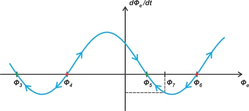
Figure 5. Following the phase-plane trajectory when the initial phase is ϕ₇.

 

Since dϕ_e/dt is negative, the loop decreases the phase error (ϕ_e) as time passes. This causes the system to move away from ϕ₆ and toward ϕ₅. Conversely, when the initial phase lies between ϕ₄ and ϕ₅, where dϕ_e/dt is positive, the loop increases ϕ_e over time. This makes the system transition away from ϕ₄ and toward ϕ₅. Thus, ϕ₅ is a stable point because the system moves towards it when the initial phase is above or below ϕ₅.

Similarly, we can use Figure 5 to identify the transition direction for the other phase error intervals. Note that the system tries to move away from points ϕ₄ and ϕ₆, indicating that these are the system's metastable points. While the system can instantaneously reach equilibrium at the metastable points, a small perturbation—noise, for example—will move the operating point away from these points.

Before continuing, note that when the loop locks at a point like ϕ₅, the VCO oscillates at the input frequency. However, there is a non-zero phase error of ϕ₅ between the incoming signal and the VCO output.

 

Maximum Frequency Step of a First-Order PLL

We observed that the phase-plane plot of a first-order PLL is a vertically shifted sinusoid, and the points where the plot intersects the zero level define the system's equilibrium points. In the examples above, the plot intersected the horizontal axis, indicating the presence of equilibrium points in the system.

However, this is not always the case. According to Equation 17, the plot does not cross the horizontal axis when Δ⍵ > K₀. This is illustrated in Figure 6.

 

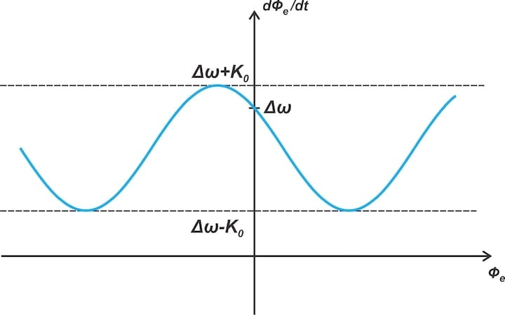
Figure 6. Typical phase-plane plot of a first-order PLL when the input frequency step is greater than K₀.

 

When Δ⍵ > K₀, the loop never achieves lock, and the phase error (ϕ_e) proceeds along the phase-plane trajectory forever. Thus, a first-order PLL can lock only if the difference between the incoming frequency and the VCO's quiescent frequency is less than K₀.

 

Wrapping Up

A first-order PLL can lock only if the frequency difference between the incoming signal and the VCO's quiescent frequency is less than the gain factor (K₀). When lock is achieved, the first-order PLL exhibits a non-zero phase error between the incoming signal and the VCO output. Higher-order PLLs address these issues, but they also introduce stability challenges.

 

This article is Part 2 of a 12-part series on loop filters in PLL design. All articles in this series are listed below in order of publication:

1. Foundations for PLL Nonlinear Analysis: Modeling the Phase Detector and VCO
2. Analyzing a First-Order PLL in Acquisition Mode With a Nonlinear Model
3. Analyzing First-Order PLLs Using Linear Models
4. Understanding the Limitations of the First-Order PLL
5. Introduction to Second-Order Type-1 PLLs
6. Understanding the Limitations of the Second-Order Type-1 PLL With a Lag Filter
7. Analyzing the Lag Filter’s Effect on PLL Performance
8. Introducing the Lag-Lead Filter
9. Exploring the Bode Plots of PLLs With a Lag-Lead Loop Filter
10. Understanding the Time-Domain Response of PLLs With Lag-Lead Filters
11. Introduction to Second-Order Type-2 PLLs
12. Second-Order Type-2 PLLs: Bode Diagrams, Bandwidth, and Overshoot

 

All images used courtesy of Steve Arar