Understanding SNR in DSB‑SC Coherent Detection: A Graphical Approach

In the previous article, we examined how coherent detection influences signal and noise transformation in the DSB‑SC method, focusing primarily on a mathematical treatment. In this article, we shift to a graphical illustration to help you quickly visualize how signal and noise power evolve under DSB‑SC coherent detection, providing a more intuitive perspective alongside the earlier analytical approach. To fully grasp the forthcoming discussion, it’s essential to first examine how correlated and uncorrelated signals combine.

 

Comparing the Power of Coherently vs. Incoherently Added Signals

When two signals of the same frequency are combined, the resulting power depends on whether they are deterministic or statistically independent. Consider first the simple case of two coherent, phase‑aligned signals, for example x(t) = y(t) = A·cos⁡(ω_ct). Adding these signals produces 2A·cos⁡(ω_ct). In this situation, the amplitude is doubled, resulting in a fourfold increase in power relative to each component, since power scales with the square of the amplitude.

In contrast, if the two signals are statistically independent, their powers add rather than their amplitudes, resulting in a total power that is only twice that of each component. Suppose x(t) and y(t) are two statistically independent random signals. The average power of their sum is given by:

$$\begin{eqnarray} P_{tot} &=& \lim_{T \rightarrow \infty} \frac{1}{T} \int_{-T/2}^{T/2} [x(t) + y(t)]^2 \ dt \\ &=& \lim_{T \rightarrow \infty} \frac{1}{T} \int_{-T/2}^{T/2} [x^{2}(t) + y^{2}(t) + 2x(t)y(t)] \ dt \end{eqnarray}$$

Equation 1.

 

The time averages of x²(t) and y²(t) clearly correspond to the average powers of the input signals. But what does the third term in the integral represent? The final term represents the correlation between the two signals, reflecting the degree of similarity between them. For statistically independent signals, the correlation is zero, so the last term vanishes. In this case, the total power is simply the sum of the individual powers. This contrasts with the coherent, phase‑aligned signals, which yielded a fourfold increase in output power when combined.

Formally, for statistically independent functions, the average of their product equals the product of their averages. If the signals are zero‑mean, the cross‑term disappears, and the output power is simply the sum of the individual powers. Figure 1 helps you visualize how combining correlated, phase‑aligned signals yield greater output power compared to uncorrelated signals.

 

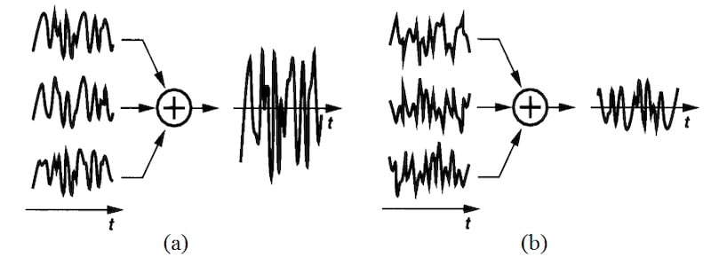
Figure 1. Combining correlated, phase-aligned signals (a) yields higher output power compared to uncorrelated signals (b). Image used courtesy of B. Razavi.

 

Having established how coherent and incoherent signals combine, we’re now prepared to examine the noise performance of the DSB‑SC coherent detector.

 

Brief Overview of the DSB-SC Method

To generate a DSB-SC signal, the message signal m(t) is multiplied by the carrier wave A·cos⁡(2πf_ct), yielding:

$$s(t) = m(t) \times A_c cos(\omega_c t)$$

Equation 2.

 

As shown in Figure 2, the message is often a lowpass signal of bandwidth W, implying that virtually no power is present at frequencies above W.

 

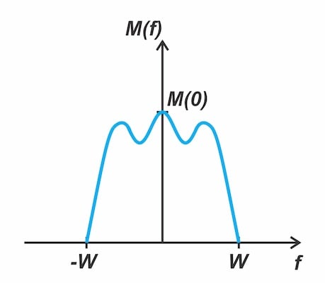
Figure 2. The spectrum of the message signal has zero power for |f|>W.

 

An important concept, which provides the foundation for understanding the modulated signal’s spectrum and the subsequent noise analysis in this article, is how multiplication by cos⁡(2πf_ct) transforms the signal’s spectral content.

When a spectral component at frequency f₁ is multiplied by cos(2πf_ct), the result is two new frequency components at f₁±f_c. Each new component inherits half the amplitude of the original, and thus carries one-fourth of its power. Therefore, the frequency spectrum of the modulated signal s(t) is as shown in Figure 3.

 

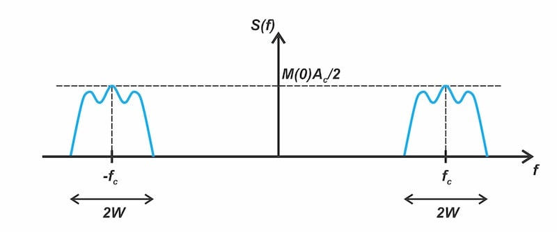
Figure 3. Typical spectrum of a DSB-SC signal.

 

To demodulate s(t), the receiver multiplies it by a locally generated carrier wave cos⁡(2πf_ct) that is phase-coherent with the original carrier used in the transmitter. Shown in Figure 4 is the basic block diagram of a coherent detector.

 

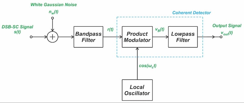
Figure 4. The model of a DSB-SC receiver for coherent AM detection.

 

In the rest of the article, we'll explore how the output signal and noise power relate to the signal and noise power present at the demodulator’s input.

 

Calculation of Output Signal Power

When the positive-frequency portion of s(t) shown in Figure 3 is multiplied by cos⁡(2πf_ct), two spectral components emerge: one centered at DC and the other around 2f_c, as illustrated in Figure 5.

 

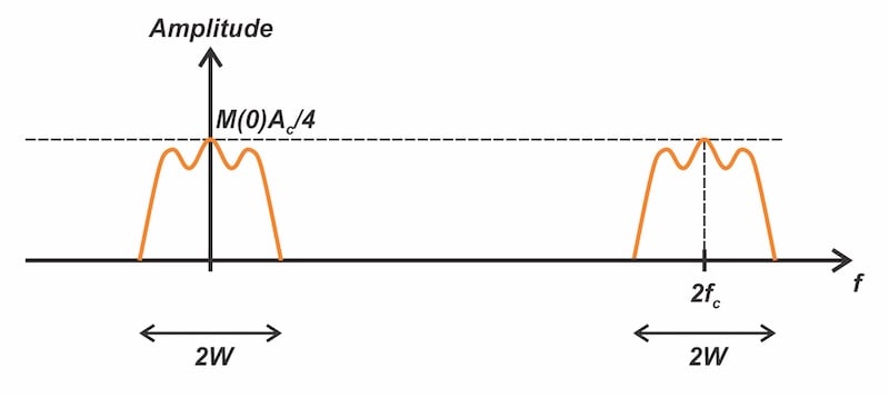
Figure 5. Spectrum resulting from multiplying the positive-frequency portion of s(t) by the carrier wave.

 

Note that the amplitude of each frequency component is scaled by a factor of 0.5. Similarly, multiplying the negative-frequency component of s(t) by the carrier wave yields the spectrum shown in Figure 6.

 

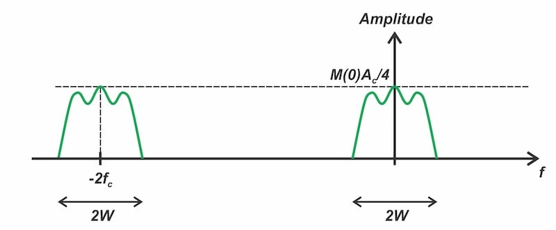
Figure 6. Spectrum resulting from multiplying the negative-frequency portion of s(t) by the carrier wave.

 

The lowpass filter following the multiplier suppresses the high-frequency components around 2f_c, allowing only the baseband content near DC to pass through. A natural follow-up is to ask how the baseband components in Figures 5 and 6 combine to form the output signal. We can show that the two baseband components are in phase and hence their superposition leads to an output amplitude twice that of either component alone, producing the spectrum shown in Figure 7.

 

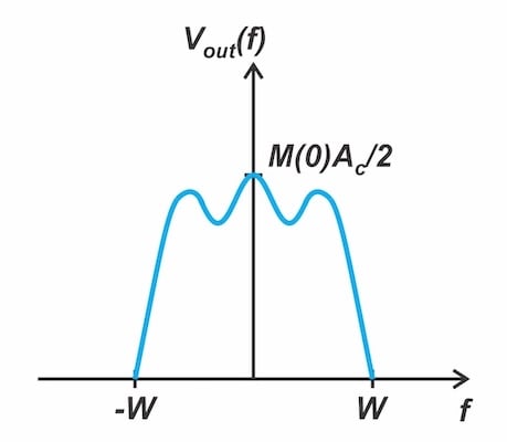
Figure 7. The spectrum of the output signal.

 

Comparing the input and output spectra in Figures 3 and 7, we observe that the signal at the input of the demodulator contains two replicas of the message spectrum, whereas the output retains only one. Since both figures have equal amplitude scaling factors, the output signal carries half the power of the input. Defining P_s,in and P_s,out as the input and output signal powers, we obtain:

$$P_{s,out} = \frac{1}{2} P_{s,in}$$

Equation 3.

 

This result is consistent with Equation 14 in the previous article, which was derived using a more detailed mathematical approach.

 

Evaluation of Output Noise Power

In DSB-SC transmission, the carrier filter must have a minimum bandwidth equal to twice the message bandwidth 2W. Therefore, the positive-frequency portion of the noise present at the carrier filter output extends over the frequency range f_c-W to f_c+W. The bandpass noise spectrum, G_n(f), is shown in Figure 8.

 

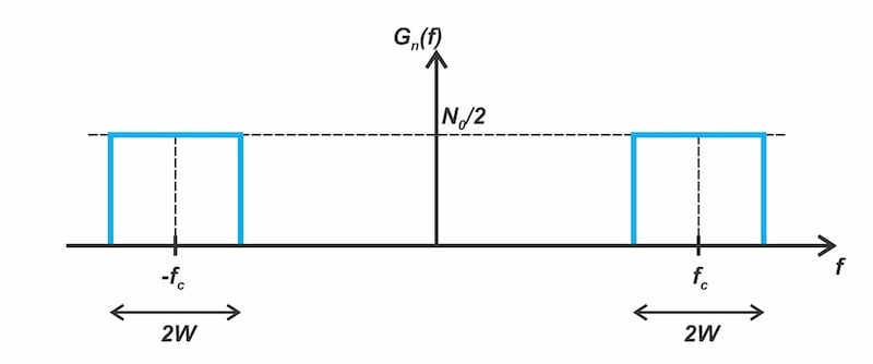
Figure 8. The noise PSD at the output of the carrier filter.

 

The average noise power equals the area under the PSD curve. Therefore, the noise power at the input of the demodulator is:

$$P_{n, in} = (\frac{N_0}{2} \times 2W) \times 2 = 2N_0 W$$

Equation 4.

 

The noise transformation resulting from multiplication by cos⁡(2πf_ct) is essentially the same as the signal transformation described earlier. Multiplying the positive-frequency portion of the PSD by cos⁡(2πf_ct) produces two components: one centered at DC and the other around 2f_c, as illustrated in Figure 9.

 

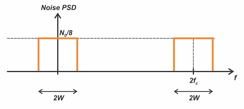
Figure 9. The noise PSD resulting from multiplying the positive-frequency portion of G_n(f) by the carrier wave.

 

Recall that the PSD is a power quantity, so the scaling factor applied to each frequency component is 0.25 instead of 0.5, which was used in our earlier discussion of signal transformation. Following the same logic, multiplying the negative-frequency portion of G_n(f) by the carrier generates the spectrum you see in Figure 10.

 

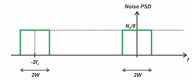
Figure 10. The noise PSD resulting from multiplying the negative-frequency portion of G_n(f) by the carrier wave.

 

After multiplication, the lowpass filter suppresses the spectral components around 2f_c, leaving only the baseband content near DC. Up to this point, the process parallels our earlier discussion of signal transformation. However, the way baseband noise components combine is distinct: because the two noise components are statistically independent, their addition doubles the output power. Recall that independent noise sources combine in terms of power rather than amplitude. This leads to the output noise PSD illustrated in Figure 11.

 

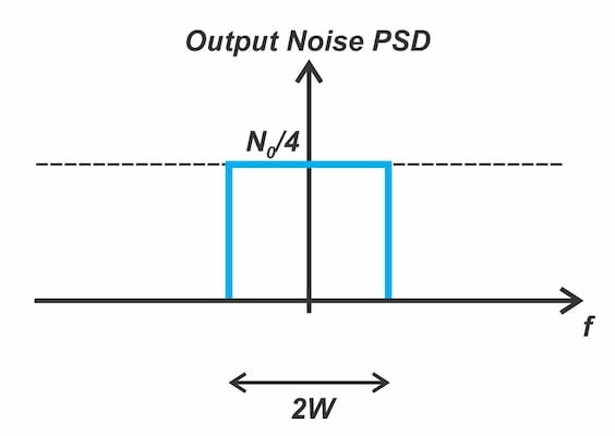
Figure 11. Output noise PSD.

 

Hence, the average noise power at the demodulator output is:

$$P_{n,out} = \frac{N_0}{4} \times 2W = \frac{1}{2}N_0 W$$

Equation 5.

 

Equations 4 and 5 can be compared to establish the relationship between the input and output noise powers:

$$P_{n,out} = \frac{1}{4} P_{n,in}$$

Equation 6.

 

The result agrees with Equation 15 from the earlier article.

 

Relationship Between Input and Output SNR

Finally, applying Equations 3 and 6 allows us to establish the relationship between the input and output SNR:

$$SNR_{out} = \frac{P_{s,out}}{P_{n,out}} = \frac{\frac{1}{2} P_{s,in}}{\frac{1}{4} P_{n,in}} = 2 \times SNR_{in}$$

Equation 7.

 

The analysis indicates that DSB‑SC demodulation doubles the SNR. In other words, the DSB-SC coherent detector offers a 3 dB improvement in SNR when comparing the input and output of the demodulator. Although signal and noise occupy the same frequency range, the signal components reinforce each other coherently during demodulation, while the noise components combine only incoherently. This difference boosts the signal power relative to the noise, producing a twofold improvement in the output SNR.

 

Wrapping Up

In this article, we revisited the noise performance of the DSB‑SC coherent detector through a graphical approach, in contrast to the previous article, which emphasized a mathematical treatment. This graphical perspective is intended to deepen understanding of the demodulation process and to provide a clear visualization of how signal and noise power behave under DSB‑SC coherent detection. In the next article, we will extend this graphical approach to examine the noise performance of the coherent SSB demodulator.