Evaluating the Noise Performance of Coherent DSB‑SC Demodulators

In earlier article collections on modulation and demodulation, we explored the fundamental principles, bandwidth requirements, and circuit-level implementations. This current series, which began with "Understanding the Characteristics of Narrowband Noise in Communication Systems," continues that discussion by examining how these systems perform in the presence of channel noise. We'll also explore how such considerations influence key design parameters, including the minimum required transmit power. As we'll see by the end of this series, modulation methods differ in their resilience to noise.

This article examines the noise performance of double-sideband suppressed-carrier (DSB-SC) communication that relies on coherent (or synchronous) detection techniques. To set the stage, let's first look at the basic properties of analog communication systems relevant to noise analysis.

 

General Model of Analog Communication Systems

Figure 1 presents a general model of analog communication systems. This model is applicable to the analysis of noise in both AM and FM schemes.

 

Figure 1. Generalized model of a continuous wave (CW) communication system used for noise analysis.

 

In the figure above, m(t) represents the message signal to be transmitted. The modulated carrier x(t) at the transmitter output is delivered to the communication channel. Except for a transmission loss of L, the channel behaves nearly ideally, introducing negligible distortion and delay.

The detector block in the receiver performs demodulation. Its configuration varies depending on the modulation scheme and the specific demodulation technique chosen for that scheme.

When a channel introduces distortion, the receiver must employ a bandpass filter with an appropriate response for equalization. The equalization filter must be placed before the detector, since demodulation is often nonlinear. The notable exception is AM synchronous detection, which operates linearly and permits equalization to happen at baseband.

While the channel is assumed to be distortionless, it's perturbed by noise. In Figure 1, the term n_w(t) represents the channel noise. It is modeled as additive white Gaussian noise with a zero mean and a double-sided power spectral density (PSD) of N₀/2 W/Hz.

The signal at the channel output, s(t), is simply added to n_w(t). The resulting composite signal is then processed by the receiver.

The bandpass filter at the receiver front end is sometimes called the carrier filter. This filter is assumed to have a unity-gain rectangular response and a bandwidth equal to the modulated wave's transmission bandwidth (B_T).

For simplicity, we use the bandpass filter to represent the entire predetection chain, which encompasses the RF and IF amplification and filtering stages within the receiver. Frequency translation and gain prior to detection are neglected in this model because they affect signal and noise equally.

Note that n_w(t) can also account for thermal noise generated within the receiver's predetection components, including the RF amplifier and subsequent IF stages. This internal noise is also modeled as additive white noise over the signal bandwidth. When including the noise from pre-detection stages, noise contributions from IF stages and mixers are typically secondary. The front-end RF amplifier provides sufficient gain to render subsequent noise sources negligible in the overall noise profile.

 

How is Noise Performance Assessed?

To evaluate the noise performance of modulation schemes, we model all significant noise sources as additive white noise at the receiver input. The attention is centered on the receiver portion of the block diagram in Figure 1. For example, Figure 2 depicts the model we use for a coherent DSB-SC demodulator.

 

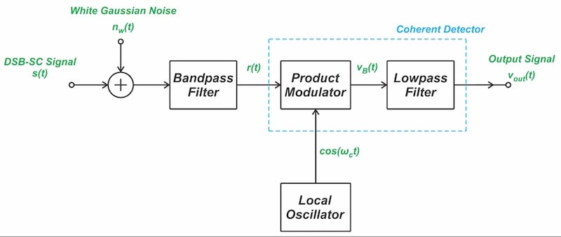
Figure 2. The model of a DSB-SC receiver for coherent AM detection.

 

In this figure, s(t) is the input signal. This is a DSB-SC AM wave with a carrier frequency of f_c and a transmission bandwidth of B_T.

Evaluating noise performance begins with constructing a mathematical model of the system components. In coherent detection, the model comprises a sequence of filtering and multiplication operations. This model allows us to track how both the input signal and noise evolve as they propagate through each stage of the demodulator.

 

Pre-Detection SNR

We'll now determine the signal-to-noise ratio (SNR) at the input of the coherent demodulator. This parameter is also known as the pre-detection SNR.

The bandpass filter has a center frequency of f_c and a bandwidth of twice the message bandwidth (2W). This allows it to pass the input AM wave without introducing any distortion. Therefore, the noisy signal presented to the detector is:

$$r(t) ~=~ s(t) ~+~ n(t)$$

Equation 1.

 

where n(t) is the noise process at the output of the filter.

The modulated signal and noise combine additively. Therefore, the input SNR can be expressed as the ratio of the average power of the modulated waveform, s(t), to that of the filtered noise, n(t). If the power in s(t) is P_s,in and the power in the input noise is P_n,in, then the pre-detection SNR is:

$$SNR_{in} ~=~ \frac{P_{s,in}}{P_{n, in}}$$

Equation 2.

 

What Is the Power of the Modulated Carrier?

First, let's calculate the power in the input signal. The double-sideband suppressed-carrier wave may be expressed as:

$$s(t) ~=~ m(t) ~\times~ A_c \cos(\omega_c t)$$

Equation 3.

 

which is calculated by directly multiplying the message signal, m(t), by the carrier wave, A_ccos(ω_ct).

We calculate the average power in s(t) as:

$$P_{s,in} ~=~ \lim_{T \rightarrow \infty} \frac{1}{T} \int_{-T/2}^{T/2} s^2(t) \ dt$$

Equation 4.

 

If s(t) were a periodic signal, calculating the integral over one period would be sufficient. However, in practice, s(t) is not usually periodic. Because of this, the measurement must be carried out over a long period.

Note that Equation 4 effectively expresses the average power delivered to a 1 Ω resistor, which is why it's sometimes called the normalized power.

Applying basic trigonometric identities, we can expand the square of the cosine function in s²(t) as follows:

$$\begin{eqnarray}P_{s, in} &~=~& \lim_{T \rightarrow \infty} \frac{1}{T} \int_{-T/2}^{T/2} m^2 (t) ~\times~ A_c^2 \cos^2 (\omega_c t) \ dt \\ &~=~& \lim_{T \rightarrow \infty} \frac{1}{T} \int_{-T/2}^{T/2} m^2 (t) ~\times~ A_c^2 \bigg (\frac{ 1 ~+~ \cos (2 \omega_c t )}{2} \bigg) \ dt \\ &~=~& \frac{1}{2}A_c^2 ~\times~ \overline{m^2(t)} \end{eqnarray}$$

Equation 5.

 

In the equation above, the bar over m²(t) denotes its time average.

You might wonder why the time average of the term involving cos⁡(2ω_ct) turns out to be zero. Intuitively, since m²(t) is a slowly varying baseband signal and cos⁡(2ω_ct) is a rapidly oscillating carrier, their product fluctuates symmetrically around zero and thus averages out over time. More formally, because the two functions are uncorrelated, the time average of their product equals the product of their individual time averages. Given that the average of cos⁡(2ω_ct) is zero, the entire term m²(t)cos⁡(2ω_ct) contributes no net power.

For notational convenience, we denote the time average of m²(t) as P_m. This yields the following expression for the average input signal power:

$$P_{s, in} ~=~ \frac{1}{2}A_c^2 ~\times~ P_m$$

Equation 6.

 

Determining the Input Noise Power

The bandpass filter at the demodulator's front end is designed with just enough bandwidth to pass the modulated signal without distortion. In DSB-SC systems, the filter's midband aligns with the carrier. Figure 3 shows the noise PSD at the output of the bandpass filter.

 

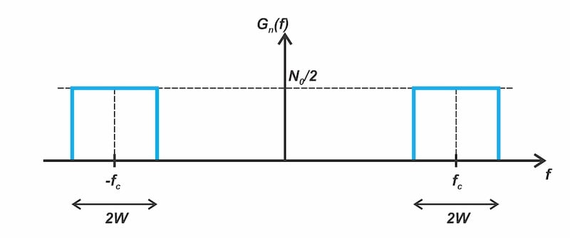
Figure 3. Noise PSD at the output of the bandpass filter.

 

The average noise power at the demodulator input equals the area under the PSD curve. For the specific PSD illustrated in the above figure, this is represented by:

$$P_{n, in} ~=~ (\frac{N_0}{2} ~\times~ 2W) ~\times~ 2 ~=~ 2N_0 W$$

Equation 7.

 

Applying Equations 6 and 7, the input SNR is given by:

$$SNR_{in} ~=~ \frac{P_{s,in}}{P_{n, in}} ~=~ \frac{A_c^2 ~\times~ P_m}{4N_0 W}$$

Equation 8.

 

Output SNR

To determine the output SNR, we need to understand how the signal and noise are transformed by the demodulator. As discussed in the previous article, the narrowband noise at the output of the bandpass filter can be represented by:

$$n(t) ~=~ n_{I}(t) \ \cos(\omega_c t) ~-~ n_{Q}(t) \ \sin(\omega_c t)$$

Equation 9.

 

where:

• n_I(t) is the in-phase noise component
• n_Q(t) is the quadrature noise component

Both noise components are measured with respect to the carrier wave A_ccos(ω_ct).

Therefore, the noisy signal that appears at the output of the bandpass filter may be expressed as:

$$r(t) ~=~ s(t) ~+~ n(t) ~=~ \big [m(t) ~\times~ A_c ~+~ n_{I}(t) \big ] \cos(\omega_c t) ~-~ n_{Q}(t) \ \sin(\omega_c t)$$

Equation 10.

 

The coherent detector multiplies the above signal by cos(ω_ct), producing:

$$v_B(t) ~=~ \big [m(t) ~\times~ A_c ~+~ n_{I}(t) \big ] \cos^2 (\omega_c t) ~-~ n_{Q}(t) \ \sin(\omega_c t) \ \cos(\omega_c t)$$

Equation 11.

 

Applying basic trigonometric identities, this simplifies to:

$$v_B(t) = 0.5\big [m(t) \times A_c + n_{I}(t) \big ] ~+~ 0.5\big [m(t) \times A_c + n_{I}(t) \big ] \cos (2\omega_c t) ~-~ 0.5 \times n_{Q}(t) \ \sin(2\omega_c t)$$

Equation 12.

 

The lowpass filter following the multiplier eliminates the double-frequency terms at 2ω_c, leaving only the baseband component.

$$v_{out}(t) ~=~ 0.5\big [m(t) ~\times~ A_c ~+~ n_{I}(t) \big ]$$

Equation 13.

 

Comparing Equations 10 and 13, we observe that an ideal synchronous detector simply extracts the in-phase component of the input signal. Also, note that the output signal and noise are additive. This allows us to derive an analytical expression for the output SNR. From Equation 13, the power of the output signal component is simply:

$$P_{s,out} ~=~ \frac{1}{4} A_c^2 ~\times~ P_m ~=~ \frac{1}{2} P_{s,in}$$

Equation 14.

 

where the second equality follows from Equation 6.

As discussed in the previous article, if the power of the bandpass noise at the input of the detector is P_n,in, then the power of each of its in-phase and quadrature components is also P_n,in. Therefore, from Equation 13, the power in the noise component of v_out(t) is:

$$P_{n,out} ~=~ \frac{1}{4} ~\times~ {[Power \ in \ n_I(t)]} ~=~ \frac{1}{4} P_{n,in}$$

Equation 15.

 

Using Equation 7, this becomes:

$$P_{n,out} ~=~ \frac{1}{2}N_0 W$$

Equation 16.

 

Now, using Equations 15 and 16, the output SNR is obtained as:

$$SNR_{out} ~=~ \frac{P_{s,out}}{P_{n,out}} ~=~ \frac{ A_c^2 ~\times~ P_m}{2N_0 W}$$

Equation 17.

 

The output SNR can be improved by increasing the transmitted signal power, narrowing the message bandwidth, or reducing receiver noise. Comparing Equations 8 and 17, we observe that the output SNR is twice the input SNR. The DSB-SC coherent detector provides a 3 dB improvement in SNR between its input and output.

 

Example: Determining Carrier Power for a Tone-Modulated DSB-SC Wave

Consider a tone-modulated DSB-SC wave with message signal given by:

$$m(t) = \cos(2π × 15000 × t)$$

In this case, the average message power is 0.5, and the message bandwidth is W = 15 kHz.

If the noise affecting the system has a two-sided PSD of N₀/2 = 10^-14 W/Hz, what carrier power should be used to achieve an SNR of 40 dB at the output of the coherent demodulator?

 

Solution

A 40 dB SNR translates to a numerical value of 10⁴. Substituting the problem data into the output SNR expression (Equation 17) produces:

$$10^{4} ~=~ \frac{ A_c^2 ~\times~ 0.5}{2 ~\times~ (2 ~\times~ 10^{-14}) ~\times~ (15 ~\times~ 10^{3})}$$

Equation 18.

 

The required carrier power, given by A_c²/2, is calculated to be 6 μW.

 

Wrapping Up

In this article, we derived the expression for the output SNR of the DSB‑SC coherent detector and highlighted the parameters that influence noise performance. Our analysis showed that the DSB‑SC coherent detector provides a 3‑dB improvement between the demodulator's input and output. While this article focused on the mathematical derivation, the next article will visualize how signal and noise power change under DSB‑SC coherent detection.