Understanding Double-Sideband Suppressed-Carrier Modulation

In the previous article in this series, we discussed the basics of modulation and its importance to communication systems. As we learned, modulation plays a pivotal role in applications, such as audio broadcasting, where analog signals need to be transmitted over long distances.

The fundamental objective of modulation is to shift a baseband signal’s frequency range to a new frequency band centered around an RF carrier frequency. The most straightforward way of accomplishing this is amplitude modulation (AM), which varies the amplitude of a sinusoidal carrier wave in accordance with the baseband signal. In this article, we’ll explore an AM variant known as double-sideband suppressed-carrier (DSB-SC) modulation in both the time and frequency domains.

 

DSB-SC Modulation in the Frequency Domain

The baseband signal, or message signal, is typically denoted by m(t). It’s a lowpass signal of bandwidth B (Figure 1). In AM broadcasting, the message signal might be music or spoken-word content.

 

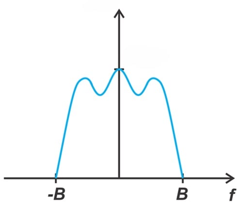
Figure 1. The frequency spectrum of an example message signal.

 

The goal of amplitude modulation is to impress the message signal on the amplitude of a carrier signal. A sinusoidal carrier wave of frequency f_c is given by:

$$c(t) ~=~ A_c \cos( \omega_c t)$$

Equation 1.

 

where A_c is the amplitude of the carrier signal and ω_c is its frequency in radians per second.

There are several ways of encoding the message onto the carrier wave’s amplitude, each with its own advantages and disadvantages. From a mathematical point of view, the simplest is to multiply m(t) by the carrier wave. Substituting Equation 1 for c(t), we obtain the following equation for the modulated signal:

$$s(t) ~=~ m(t) ~\times~ A_c \cos(\omega_c t)$$

Equation 2.

 

In the frequency domain, multiplication of m(t) by the carrier wave corresponds to a convolution of the baseband signal's spectrum, M(f), with the spectrum of the cosine function.

The spectrum of A_ccos(⍵_ct) consists of two impulse functions at ±f_c, each with an amplitude of 0.5A_c. The spectrum of the modulated wave, S(f), therefore has two copies of the baseband spectrum: one shifted to f_c and the other to –f_c. This gives us the following equation:

$$S(f) ~=~ \frac{A_c}{2} \Big [M(f~-~f_c)~+~M(f~+~f_c) \Big ]$$

Equation 3.

 

Because m(t) is a real signal, its spectrum is symmetric around the origin (f = 0). Since multiplying by the sinusoidal carrier wave shifts the spectrum of the message signal both to the right and left by f_c, the high-frequency replicas of the baseband spectrum are also symmetric around f_c and –f_c.

Figure 2 illustrates the DSB-SC modulation process in the frequency domain. The frequency components that lie at frequencies higher than the carrier frequency (|f| > f_c) are referred to as the upper sideband (USB). Similarly, the frequency content corresponding to frequencies lower than the carrier frequency (|f| < f_c) is known as the lower sideband (LSB).

 

Figure 2. Multiplication in the time domain corresponds to a convolution of the baseband spectrum with the carrier in the frequency domain (top). This translates the baseband spectrum by ±f_c (bottom).

 

While the baseband signal has a bandwidth of B, the modulated signal spans a bandwidth of 2B, centered around the positive and negative carrier frequencies (f_c and –f_c). Meanwhile, the symmetry of the message signal around the origin means that each of the two sidebands fully contains the message information. This is what’s known as double-sideband (DSB) amplitude modulation, a name that reflects the redundancy inherent to transmitting the same message information via both the lower and upper sidebands.

To understand the “SC” part of DSB-SC, note the purple impulse functions in the upper right of Figure 2. These are the impulses associated with the sinusoidal carrier. If you examine the lower half of Figure 2, you’ll see that they don’t appear in the spectrum of the modulated signal.

We call this “suppressed-carrier” modulation, or SC for short, to distinguish it from amplitude modulation methods like the one in Figure 3 where the carrier wave is present in the output spectrum.

 

Figure 3. With some variants of amplitude modulation, the carrier wave (the purple impulses) is present in the output spectrum.

 

The carrier can consume a significant portion of the transmitted power. Because the carrier wave itself doesn’t contain any information, transmitting it along with the information-bearing sidebands is less power-efficient than the DSB-SC method.

 

DSB-SC Modulation in the Time Domain

To understand the properties of the DSB-SC modulation in the time domain, consider the example message and carrier waves in Figure 4. These waves are once again denoted by m(t) and c(t), respectively.

 

Figure 4. Example message (top) and sinusoidal carrier (bottom) waves.

 

By multiplying m(t) and c(t) together, we obtain the rapidly varying modulated waveform in Figure 5.

 

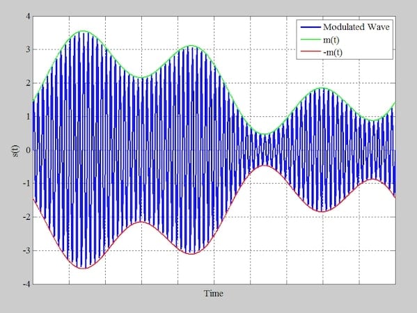
Figure 5. DSB-SC modulated wave (blue), message signal (green), and inverted message signal (red).

 

In this figure, the blue waveform represents the modulated wave. The original message signal, m(t), is shown in green; its inverted form, –m(t), is shown in red. This message signal and its inverted counterpart are identical to the upper and lower envelope of the modulated waveform, respectively. The term “envelope” refers to a continuous, smooth curve that traces the instantaneous peaks of a waveform.

Note that the message signal we’ve been examining is always greater than zero. As we’ll see in the next section, things get a bit less neat when that isn’t the case.

 

DSB-SC Modulation and Envelope for Negative Signals

The top half of Figure 6 shows a message signal that’s negative for a portion of the time shown.

 

Figure 6. Example message signal that dips below zero (top) and sinusoidal carrier wave (bottom).

 

Figure 7 shows its corresponding modulated waveform.

 

Figure 7. DSB-SC modulated wave (blue), message signal (green), and the inverted message wave (red).

 

In this example, the upper envelope of the DSB-SC signal doesn’t correspond directly to the message signal when the message signal crosses zero. Instead, as we see in Figure 8, a phase reversal occurs.

 

Figure 8. Magnified view of the phase reversal due to a sign change in m(t).

 

Because of this phase reversal, a simple envelope detector can’t be used in the receiver to restore the message signal. Instead, we need to use more complicated demodulator circuits such as the Costas loop. However, that’s a topic for a different day. For now, we’ll wrap up our discussion by working through a brief example problem.

 

Example: DSB-SC Modulation of a Single-Tone Input

Let’s apply what we’ve learned by finding the output spectrum of a DSB-SC modulated signal. To keep things simple, we’ll say that the message signal is a sinusoidal, single-tone input with frequency f_m:

$$m(t)~=~A_m \cos(2 \pi f_m t)$$

Equation 4.

 

The spectrum of this single-tone baseband signal consists of two impulses at ±f_m:

$$M(f)~=~\frac{A_m}{2} \Big [ \delta(f~-~f_m)~+~\delta(f~+~f_m) \Big ]$$

Equation 5.

 

The DSB-SC modulation translates the baseband spectrum by ±f_c and scales the spectrum by a factor of A_c/2, producing the output spectrum in Figure 9.

 

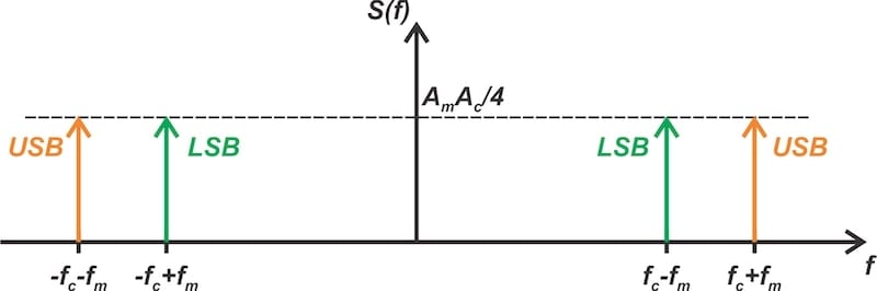
Figure 9. The output spectrum when the message signal is a cosine function at f_m.

 

We can see that the output spectrum comprises impulse functions at (f_c ± f_m) and (–f_c ± f_m).

 

Wrapping Up

For ease of reference, the key takeaways from this article are summarized below:

• Due to the symmetry of the message signal, the sidebands of the DSB-SC modulated signal are mirror images of each other around the carrier frequency. As a result, either sideband can be used to reconstruct the message signal.
• With DSB-SC modulation, the output spectrum doesn’t contain a carrier component. In other words, all the transmitted power is contained in the frequency-shifted replicas of the message signal.
• Because the envelope of the DSB-SC wave doesn’t always correspond to the message signal, envelope detector circuits can’t be used to demodulate DSB-SC signals.

In the next article, we’ll examine an amplitude modulation technique that sacrifices some of DSB-SC’s power efficiency in exchange for making demodulation simpler.

 

This article is Part 2 of a series on amplitude modulation in RF systems. A complete list of articles in this series is provided below:

1. Introduction to Modulation Techniques in RF Systems
2. Understanding Double-Sideband Suppressed-Carrier Modulation
3. Understanding Conventional Amplitude Modulation
4. Understanding the Square-Law Modulator for Generating AM Signals
5. Introduction to the Balanced Modulator for AM Signals
6. How Do Switching Modulators Generate AM Signals?
7. Understanding How Ring Modulators Produce AM Signals
8. Four Interesting AM Modulation Circuits You Should Know About
9. Demodulating Double-Sideband AM Signals
10. Introduction to Single-Sideband Modulation: The Filter Method
11. The Phasing Method and Hilbert Transforms for Single-Sideband Modulation
12. A Visual Approach to Understanding the Phasing Method for SSB Modulation
13. How Phasors Help Us Understand Bandpass Signals
14. Introduction to Weaver’s Method for SSB Signal Generation
15. Exploring the Operation of the Weaver Modulator for Single-Sideband Modulation

 

All images used courtesy of Steve Arar