Understanding the Square-Law Modulator for Generating AM Signals

As we learned in the first article of this series, modulation moves input frequencies to a different range at the output. Systems that are both linear and time-invariant can’t generate frequencies other than those in the input signal. Modulator circuits must, therefore, be nonlinear, time-varying, or both.

Square-law modulators fall into the “both” category. In this article, we’ll learn the basics of how square-law modulators generate AM signals. As we’ll see, nonlinearity plays a key role in the design of these circuits.

 

The Conventional AM and DSB-SC Techniques

Before anything else, let's briefly review the equations for double-sideband suppressed-carrier (DSB-SC) and conventional AM modulation. In DSB-SC modulation, the modulated signal is generated by multiplying the message signal (m(t)) by the carrier wave (c(t) = A_ccos(ω_ct)):

$$s_{out}(t) ~=~ m(t) ~\times~ A_c \cos(\omega_c t)$$

Equation 1.

 

To ensure the carrier wave remains in the transmitted spectrum, conventional AM employs the following equation to produce the modulated signal:

$$s_{out}(t) ~=~ A_c \Big ( 1~+~ \mu m(t) \Big ) \cos(\omega_c t)$$

Equation 2.

 

In both cases, we could use an analog multiplier to directly compute the output signal. The square-law modulator is another common way of implementing this multiplication.

 

How a Square-Law Modulator Generates AM Signals

The core idea of the square-law modulator is that the square of the sum of two functions generates a cross-product term proportional to the product of the two functions. Assume that the input-output characteristic of a nonlinear device can be represented by:

$$y(t) ~\approx~ \alpha_1 x(t) ~+~ \alpha_2 x^2(t)$$

Equation 3.

 

If we add the message (m(t)) and carrier (c(t) = cos(⍵_ct)) waves together and pass the combined signal through the above square-law characteristic, we get:

$$y(t) ~\approx~ \alpha_1 m(t) ~+~ \alpha_2 m^2(t) ~+~ \alpha_2 \cos^2( \omega_c t) ~+~ \Big ( \alpha_1 ~+~ 2 \alpha_2 m(t) \Big ) \cos( \omega_c t)$$

Equation 4.

 

The last term in the above equation is the desired AM wave. Equation 5 rewrites this term for ease of comparison with the conventional AM signal in Equation 2:

$$s_{out} ~=~ \alpha_1 \Big ( 1 ~+~ 2 \frac{ \alpha_2}{\alpha_1} m(t) \Big ) \cos( \omega_c t)$$

Equation 5.

 

The signal uses a modulation index of:

$$\mu~=~2 \frac{ \alpha_2}{\alpha_1}$$

Equation 6.

 

But how do we separate the desired AM wave from the other spectral components? Let’s explore this question in the next section.

 

Extracting the AM Signal

Assume that m(t) is a lowpass signal with bandwidth B as shown in Figure 1.

 

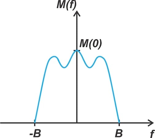
Figure 1. The spectrum of the message signal has zero power for |f| > B.

 

Let's determine the frequency range of the other components in Equation 4.

First, we examine the bandwidth of m²(t), the square of the message signal. When we square m(t), we’re essentially multiplying the signal by itself in the time domain.

According to the convolution theorem, multiplication in the time domain corresponds to convolution in the frequency domain. If M(f) is the Fourier transform of m(t), then the Fourier transform of m²(t) is the convolution of M(f) with itself (M(f)*M(f)). Due to the basic properties of convolution, we also know that the bandwidth of M(f)*M(f) is twice the bandwidth of M(f). This is illustrated in Figure 2.

 

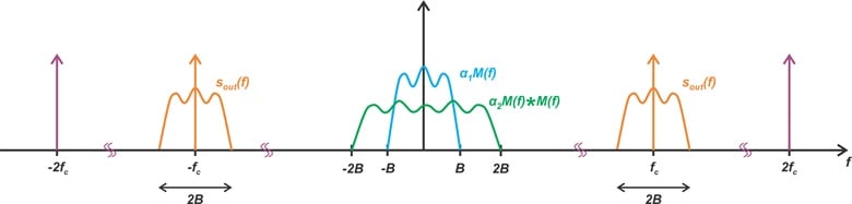
Figure 2. The output spectrum of a nonlinear device with a square-law characteristic.

 

We can interpret this figure as follows:

• The spectrum of the message signal (m(t)) is shown in blue.
• The green spectrum shows the frequency range occupied by m²(t).
• The spectrum of the desired signal (s_out) is shown in orange.
• The purple impulse functions are created by the square of the carrier wave (cos²(⍵_ct)).

The exact shape of the spectrum of m²(t) isn’t our concern here. What’s important is that its Fourier transform is confined to frequencies below 2B Hz.

Provided that its spectrum doesn’t overlap with those of m(t) and m²(t), the desired signal can be separated from the other terms using a bandpass filter. From Figure 2, the condition for avoiding spectral overlap is:

$$f_c ~-~ B ~\geq~ 2B ~\rightarrow~ f_c ~\geq~ 3B$$

Equation 7.

 

In the real world, the ratio of the carrier frequency to the baseband signal’s bandwidth (f_c/B) is typically 100 to 300, so it’s easy to meet this condition. We can, therefore, use a square-law device followed by a bandpass filter (Figure 3) to generate AM waves.

 

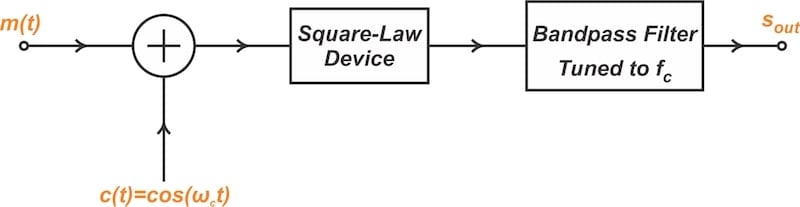
Figure 3. Block diagram of a square-law modulator.

 

The bandpass filter is tuned to the carrier frequency (f_c) and ideally has a bandwidth of 2B. Figure 2 shows that the filter should have a transition band of (f_c – B) – 2B ≈ f_c to suppress the spectrum component around zero frequency.

Some AM modulators require a less stringent transition band of about 2f_c because their structure eliminates the spectrum component centered at f = 0. With these modulators, the closest undesired spectrum is centered at 3f_c. However, that’s a discussion for another day. For now, let’s look at a few practical examples of square-law modulators.

 

Practical Circuit Implementations

The nonlinear device in a square-law modulator can be a semiconductor diode, a BJT, or a FET device. Due to their poor noise performance, however, diodes aren’t very common. Bipolar transistors also have drawbacks, as they generate high levels of spurious frequencies that need filtering. Figure 4 shows the basic schematic of a square-law modulator built around a BJT device.

 

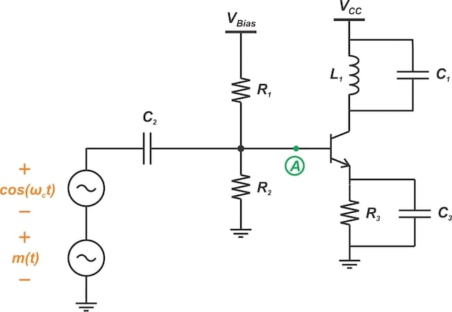
Figure 4. A square-law modulator using a BJT as the nonlinear device.

 

In this implementation, the transistor provides the nonlinearity and the LC circuit filters out the higher harmonic components.

 

FET Implementations

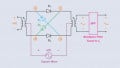
FETs are preferred for square-law modulation due to their nearly square-law input-output characteristic. Figure 5 illustrates a FET implementation that employs a transformer to combine the carrier with the message signal.

 

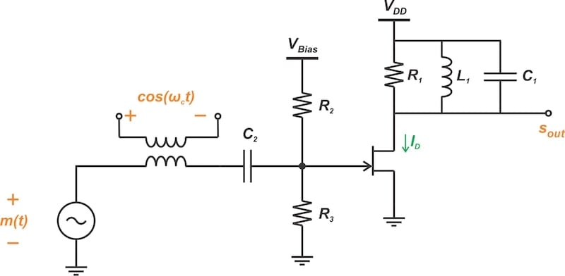
Figure 5. A FET-based square-law modulator.

 

Based on the superposition principle, we can also use two resistors to generate the sum of m(t) and the carrier wave. Figure 6 shows a FET square-law modulator that uses this method. The bias circuit is not shown.

 

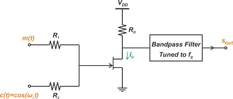
Figure 6. A resistive network can be used to generate the sum of the message and carrier waves.

 

Generating DSB-SC Signals Using a Square-Law Modulator

We’ve seen that a square-law modulator can generate conventional AM signals, but what about DSB-SC signals? As it turns out, a square-law modulator can generate DSB-SC signals if the input-output characteristic of the device doesn’t have a linear term—in other words, if ⍺₁ = 0 in Equation 3. In this case, the signal at the output of the bandpass filter is:

$$s_{out} ~=~ 2 \alpha_2 m(t) \cos( \omega_c t)$$

Equation 7.

 

With practical devices, ⍺₁ is typically non-zero. To generate DSB-SC signals, we can incorporate two square-law modulators in a balanced configuration. This balanced arrangement also reduces the undesired effect of higher-order nonlinearity terms on the performance of the modulator, as we’ll discuss in the next article of this series.

 

Wrapping Up

A square-law modulator generates AM waves by adding the message signal and carrier signal, then passing the combined signal through a nonlinear device and a bandpass filter. If both the linear (⍺₁) and second-order (⍺₂) terms are non-zero, the carrier appears at the output, generating conventional AM waves. If ⍺₁ = 0, the carrier isn’t present at the output and a DSB-SC signal is generated.

We can also use two square-law devices in a balanced configuration to generate DSB-SC signals. An important advantage of the balanced modulator is that it eliminates the undesired terms produced by the cubic nonlinearity, which is significant in most electronic components. In view of the heavy filtering required, square-law modulators are used primarily for relatively low-power modulation.

 

This article is Part 4 of a series on amplitude modulation in RF systems. A complete list of articles in this series is provided below:

1. Introduction to Modulation Techniques in RF Systems
2. Understanding Double-Sideband Suppressed-Carrier Modulation
3. Understanding Conventional Amplitude Modulation
4. Understanding the Square-Law Modulator for Generating AM Signals
5. Introduction to the Balanced Modulator for AM Signals
6. How Do Switching Modulators Generate AM Signals?
7. Understanding How Ring Modulators Produce AM Signals
8. Four Interesting AM Modulation Circuits You Should Know About
9. Demodulating Double-Sideband AM Signals
10. Introduction to Single-Sideband Modulation: The Filter Method
11. The Phasing Method and Hilbert Transforms for Single-Sideband Modulation
12. A Visual Approach to Understanding the Phasing Method for SSB Modulation
13. How Phasors Help Us Understand Bandpass Signals
14. Introduction to Weaver’s Method for SSB Signal Generation
15. Exploring the Operation of the Weaver Modulator for Single-Sideband Modulation

​​​​​​​

All images used courtesy of Steve Arar