How Phasors Help Us Understand Bandpass Signals

Bandpass signals and systems are crucial in communication systems. Interestingly, all the information carried in a real-valued bandpass signal is contained in a corresponding complex-valued baseband signal. This complex baseband representation is extremely helpful for understanding radio communication systems.

In this article, we’ll learn about the complex baseband representation of bandpass signals. As part of this discussion, we’ll also explore the concept of phasor analysis in AC circuits. Before we dive in, however, let’s make sure we’ve covered the basics by reviewing the definition of lowpass and bandpass signals.

 

Lowpass and Bandpass Signals

A signal is termed a lowpass signal when its frequency content or spectrum is centered around zero frequency. In other words, a lowpass signal has a well-defined bandwidth B with negligible spectral content for |f| > B.

 

Figure 1. The real (a) and imaginary (b) parts of a real-valued lowpass signal with bandwidth B.

 

Note that if s(t) is a real-valued function, its Fourier transform (S(f)) will exhibit conjugate symmetry. This means the real part of S(f) is an even function, whereas the imaginary part is an odd function.

A bandpass signal, on the other hand, has its spectrum centered at a frequency (f_c) that is much larger than the signal bandwidth (B). Figure 2 shows the real and imaginary parts of an example bandpass signal.

 

Figure 2. The spectrum of a real-valued bandpass signal with center frequency f_c and bandwidth B, separated into the real (a) and imaginary (b) parts.

 

Like the example baseband spectrum in Figure 1, Figure 2 exhibits conjugate symmetry due to the signal being real-valued.

The bandwidth of a real signal is defined as the span of all positive frequency components contained within the signal. If the highest and lowest positive frequencies present in the signal are, respectively, f_max and f_min, then the signal’s bandwidth is:

$$B~=~ f_{max} ~-~ f_{min}$$

Equation 1.

 

According to the above definition, the bandwidth of a single-tone sinusoid at frequency f_c and with constant amplitude A is zero.

$$s(t) ~=~ A \cos( \omega_c t ~+~ \theta)$$

Equation 2.

 

However, if A varies slowly with time, then we have an amplitude-modulated (AM) wave with a non-zero bandwidth.

 

Phasor Representation In AC Circuits

A phasor is a complex number that represents the magnitude and phase angle of a sinusoidal waveform. In AC circuit analysis, phasors are used to analyze frequency-dependent effects.

For example, consider the single-tone sinusoidal wave shown in Equation 2. This signal is the real part of a complex function:

$$s(t) ~=~ Re \Big \{ \big [A e^{j \theta} \big ] e^{j \omega_c t} \Big \}$$

Equation 3.

 

where the operator Re{.} denotes the real part of the quantity enclosed inside the curly brackets. We can represent the term inside the curly brackets as a vector in the complex plane with amplitude A and initial phase θ. As shown in Figure 3, this signal rotates around the origin at an angular velocity of ⍵_c = 2πf_c.

 

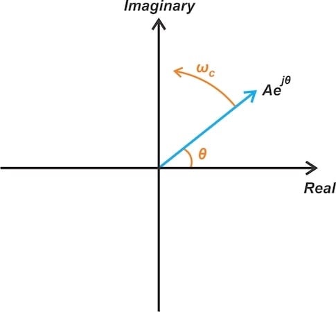
Figure 3. Phasor representation of a single-tone sinusoidal wave.

 

The projection of the above vector on the real axis (its real part) produces the original signal shown in Equation 2. The angular term ω_ct represents a steady counterclockwise rotation at f_c revolutions per second. To obtain a simplified representation of the signal, we’ll temporarily ignore this term.

Removing the rotation leads to a fixed vector that corresponds to the term inside the square brackets in Equation 3. This term, which is independent of time, is the phasor associated with our signal. It’s given by:

$$s_l ~=~ A e^{j \theta}$$

Equation 4.

 

To understand the significance of the phasor representation, consider a linear time-invariant (LTI) system excited by a sinusoidal input. As illustrated in Figure 4, this excitation produces sinusoidal signals at all nodes within the circuit. Though all of these signals have the same frequency, they may differ in amplitude and phase.

 

Figure 4. Sinusoidal signals produced by an LTI circuit can be described by phasors that have different amplitudes and initial phases but rotate at the same angular velocity.

 

Since all these vectors rotate at the same velocity, the phase difference between them doesn’t change with time. The amplitude ratios of these vectors are likewise independent of time. Thus, we can freeze the rotating vectors at a specific moment in time.

Removing the time dependence from the voltage and current quantities allows us to represent them as complex-valued, time-independent numbers. This significantly simplifies the circuit analysis. Once we’ve calculated the vector for a voltage or current quantity, we can reintroduce the rotating aspect to determine the actual time-domain expression for the quantity.

In short, phasors strip away the complexity of time-dependence, making it easier to describe voltage and current quantities. Loosely speaking, you could view the phasor as the lowpass or DC equivalent of a single-frequency sinusoidal wave.

 

Deriving the Lowpass Equivalent of a Modulated Bandpass Signal

So far, we’ve assumed the sinusoidal wave had a fixed amplitude and phase. However, a similar analysis can be applied to a sinusoidal wave at a fixed frequency f_c with a slowly varying amplitude and phase. Let the modulated wave centered at ⍵_c be defined as:

$$s_{RF}(t) ~=~ A(t) \cos \big ( \omega_c t ~+~ \theta(t) \big )$$

Equation 5.

 

where A(t) and θ(t) are the instantaneous amplitude and phase of the time-varying signal. The above equation can be rewritten as:

$$s_{RF}(t) ~=~ Re \Big \{ \big [A(t) e^{j \theta(t)} \big ] e^{j \omega_c t} \Big \}$$

Equation 6.

 

Equation 7 separates out the term inside the brackets:

$$s_l (t) ~=~ A(t) e^{j \theta(t)}$$

Equation 7.

 

This term is the complex baseband representation of the bandpass signal. The above equation can also be expressed in Cartesian form:

$$s_l(t) ~=~ s_i(t) ~+~ j s_q (t)$$

Equation 8.

 

where s_i(t) and s_q(t) are the real-valued in-phase and quadrature components of the equivalent baseband signal s_l(t). These components are given by:

$$s_i(t) ~=~ A(t) \cos ( \theta) \quad \text{and} \quad s_q(t)~=~A(t) \sin( \theta)$$

Equation 9.

 

Because the in-phase and quadrature components of a bandpass signal are slowly varying, we know that they’re both lowpass signals. Substituting the Cartesian form of s_l(t) into Equation 6, we can express the original RF wave in terms of its in-phase and quadrature components:

$$s_{RF}(t) ~=~ s_i(t) \cos( \omega_c t) ~-~ s_q (t) \sin( \omega_c t)$$

Equation 10.

 

The above equation shows that a bandpass signal can be represented in terms of two lowpass signals, specifically its in-phase and quadrature components.

 

The Equivalent Lowpass Signal: A Visual Representation

The complex lowpass representation of a bandpass signal can be viewed as a time-varying phasor with its starting point at the origin of the (s_I-s_Q) complex plane. This is illustrated in Figure 5.

 

Figure 5. The equivalent baseband signal, s_l(t), represented as a time-varying phasor in the (s_I-s_Q) plane.

 

Since the in-phase and quadrature components (s_i(t) and s_q(t), respectively) are functions of time, the end of the phasor vector moves about in the (s_I-s_Q) plane.

From Equation 6, we observe that the equivalent baseband signal, s_l(t), is multiplied by the complex exponential exp(jω_ct) to produce the bandpass signal s_RF(t). Therefore, the vector s_l(t) as well as the (s_I-s_Q) plane rotate at an angular velocity of ⍵_c = 2πf_c.

 

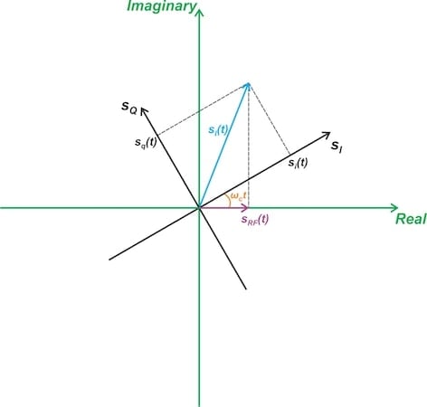
Figure 6. The time-varying phasor in the complex plane with the rotation aspect included.

 

The original bandpass signal s_RF(t) is the projection of this time-varying phasor onto a fixed line representing the real axis.

 

Reconstructing the Bandpass Signal

Equation 10 immediately tells us how we can reconstruct the bandpass signal from the in-phase and quadrature components. The circuit for lowpass-to-passband conversion is shown in Figure 7.

 

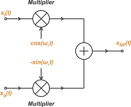
Figure 7. The block diagram for generating the bandpass signal from the lowpass in-phase and quadrature signals.

 

Next, we need to determine the equivalent baseband signal from the bandpass signal. We’ll start by multiplying s_RF(t) by 2cos(⍵_ct):

$$\begin{eqnarray}s_{RF}(t) ~\times~ 2 \cos( \omega_c t) ~&=&~ A(t) \cos \big (\omega_c t ~+~ \theta(t) \big ) ~\times~ 2 \cos( \omega_c t) \\~&=&~ A(t) \Big ( \cos \big ( 2\omega_c t ~+~ \theta(t) \big ) ~+~ \cos \big( \theta(t) \big ) \Big )\end{eqnarray}$$

Equation 11.

 

If we filter the signal component at twice the carrier frequency, we obtain:

$$Lowpass \big [s_{RF}(t) ~\times~ 2 \cos( \omega_c t) \big ] ~=~ A(t) \cos \big( \theta(t) \big ) ~=~ s_i (t)$$

Equation 12.

 

Similarly, multiplying s_RF(t) by –2sin(⍵_ct) produces:

$$\begin{eqnarray}s_{RF}(t) ~\times~ \big (-2 \sin( \omega_c t) \big ) ~&=&~ A(t) \cos \big (\omega_c t ~+~ \theta(t) \big ) ~\times~ \big ( -2 \sin( \omega_c t) \big ) \\~&=&~ -A(t) \Big ( \sin \big ( 2\omega_c t ~+~ \theta(t) \big ) ~-~ \sin \big( \theta(t) \big ) \Big )\end{eqnarray}$$

Equation 13.

 

Applying an appropriate lowpass filter eliminates the signal component at twice the carrier frequency, leading to:

$$Lowpass \big [s_{RF}(t) ~\times~ \big (-2 \sin( \omega_c t) \big ) \big ] ~=~ A(t) \sin \big( \theta(t) \big ) ~=~ s_q(t)$$

Equation 14.

 

Figure 8 shows how we can implement Equations 12 and 14 using a pair of multipliers and a pair of lowpass filters.

 

Figure 8. The block diagram for generating the lowpass in-phase and quadrature signals from the bandpass signal.

 

Wrapping Up

All the information in a real-valued passband signal is contained within a corresponding complex-valued baseband signal. In this article, we learned how to derive the lowpass complex equivalent of a bandpass signal, and vice versa.

It's worth noting that extending this discussion allows us to represent a bandpass filter using a complex lowpass filter. Having lowpass models for both bandpass signals and filters is of great practical importance. For instance, modern communication transceivers apply these models to digitally process complex baseband signals, reducing the need for analog processing of passband signals.

The circuits shown in Figures 7 and 8 are essential for understanding linear modulation schemes, regardless of whether they’re analog or digital. In the next article, we’ll see how the Weaver modulator incorporates these circuits to generate single-sideband AM signals.

 

This article is Part 13 of a series on amplitude modulation in RF systems. A complete list of articles in this series is provided below:

1. Introduction to Modulation Techniques in RF Systems
2. Understanding Double-Sideband Suppressed-Carrier Modulation
3. Understanding Conventional Amplitude Modulation
4. Understanding the Square-Law Modulator for Generating AM Signals
5. Introduction to the Balanced Modulator for AM Signals
6. How Do Switching Modulators Generate AM Signals?
7. Understanding How Ring Modulators Produce AM Signals
8. Four Interesting AM Modulation Circuits You Should Know About
9. Demodulating Double-Sideband AM Signals
10. Introduction to Single-Sideband Modulation: The Filter Method
11. The Phasing Method and Hilbert Transforms for Single-Sideband Modulation
12. A Visual Approach to Understanding the Phasing Method for SSB Modulation
13. How Phasors Help Us Understand Bandpass Signals
14. Introduction to Weaver’s Method for SSB Signal Generation
15. Exploring the Operation of the Weaver Modulator for Single-Sideband Modulation

​​​​​​​

All images used courtesy of Steve Arar