Understanding Conventional Amplitude Modulation

Amplitude modulation (AM) changes the amplitude of a carrier wave in proportion to a message signal. There are several types of AM, each characterized by a unique frequency spectrum and possessing its own pros and cons.

We discussed one type of amplitude modulation, known as double-sideband suppressed-carrier (DSB-SC) modulation, in a previous article. As we learned, this is a simple and power-efficient way of modulating signals for RF transmission. However, demodulating a DSB-SC signal requires the receiver to generate a carrier that’s coherent (synchronized) with the original carrier used in the transmitter. This requirement increases both the cost and the complexity of the receiver’s hardware.

The cost of synchronous demodulation can be particularly problematic in commercial broadcasting, where many receivers are in operation for every transmitter. In this article, we’ll explore an AM technique that addresses this economic concern by preserving the carrier within the modulated signal’s spectrum. This method, known as conventional AM, sacrifices some of DSB-SC’s power efficiency in exchange for simplifying the receiver’s hardware.

 

DSB-SC Modulation: A Review

Before we jump in, let’s quickly review DSB-SC modulation. In this method, the modulated signal (s(t)) is produced by multiplying the message signal (m(t)) by the carrier wave, c(t) = A_ccos(ω_ct):

$$s(t) ~=~ m(t) ~\times~ A_c \cos(\omega_c t)$$

Equation 1.

 

In the frequency domain, multiplication of m(t) by the carrier wave corresponds to a convolution of the baseband signal's spectrum, M(f), with the spectrum of the cosine function. Therefore, as illustrated in Figure 1, the spectrum of the modulated wave will have two copies of the baseband spectrum—one shifted to f_c and the other to –f_c.

 

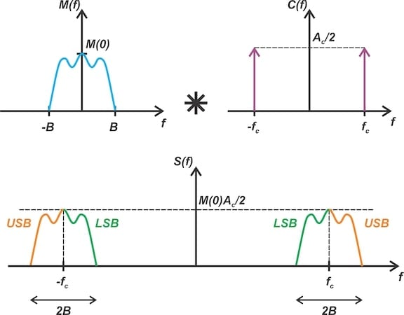
Figure 1. Multiplication in the time domain corresponds to a convolution of the baseband spectrum with the carrier in the frequency domain (top). This translates the baseband spectrum by ±f_c (bottom).

 

The key point here is that the impulse functions associated with the sinusoidal carrier (denoted by the purple vertical arrows in the upper diagram) don’t appear in the spectrum of the modulated signal. From a power-usage perspective, this is advantageous because the carrier consumes a considerable portion of the transmitted power without conveying any useful information. The downside, as we noted previously, is that it leads to increased complexity in the receiver’s hardware.

 

The Conventional AM Output Spectrum

To retain the carrier wave in the transmitted spectrum, we use the following equation to generate the modulated signal:

$$s(t) ~=~ A_c \Big ( 1~+~ \mu m(t) \Big ) \cos(\omega_c t)$$

Equation 2.

 

where:

A_c is the carrier amplitude

m(t) is the message signal

μ is the modulation index (a scaling factor).

The inclusion of 1 + in A_c(1 + μm(t)) results in the carrier wave’s presence within the output frequency spectrum.

Figure 2 shows a typical output spectrum for this type of amplitude modulation.

 

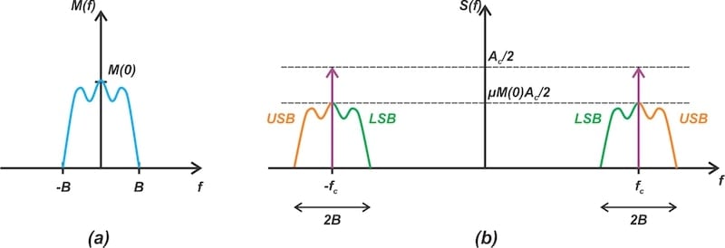
Figure 2. The spectrum of the baseband signal (a) and the conventional amplitude-modulated signal (b).

 

Comparing Figures 1 and 2, we see that the transmission bandwidth is twice that of the message signal (B_T = 2B) in both DSB-SC and conventional AM. The output spectrums of both AM types include two replicas of the baseband spectrum translated in frequency by ±f_c. However, unlike the DSB-SC method, the conventional AM spectrum includes two delta functions weighted by the factor 0.5A_c.

 

The Modulation Index in Conventional AM

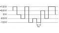
To discuss conventional AM in the time domain, we first need to understand the role of the modulation index. For example, consider a single-tone message, m(t) = cos(ω_mt), modulating the carrier wave c(t) = cos(ω_ct). Figure 3 shows the carrier wave and instantaneous amplitude of the modulated wave, g(t) = 1 + μm(t), for a modulation index of μ = 0.8.

 

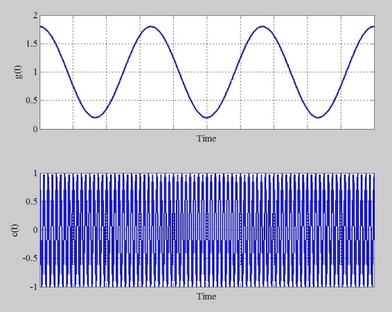
Figure 3. The function g(t) for μ = 0.8 (top) and the sinusoidal carrier wave (bottom).

 

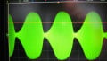
Applying Equation 2 produces the modulated waveform in Figure 4. The blue waveform in this figure represents the modulated wave; the green and red waveforms show the functions g(t) and –g(t), respectively.

 

Figure 4. The amplitude-modulated wave (blue), the function g(t) (green), and the inverted form of g(t) (red) for μ = 0.8.

 

As you may recall from the previous article's discussion of DSB-SC modulation, the envelope of a modulated signal is defined as the continuous, smooth curve that traces the instantaneous peaks of the modulated waveform. Above, the upper envelope of the modulated signal matches the function g(t), while the lower envelope of the modulated waveform is –g(t).

The function g(t) has the same shape as m(t), just offset by a DC value. Extracting m(t) from g(t) requires a DC block to eliminate the signal's DC component. Since the message information is contained in the envelope of the modulated wave, we can use a simple envelope detector circuit to restore the message.

Next, Figures 5 and 6 illustrate what happens when we increase the modulation index to μ = 1. Figure 5 shows the carrier wave and instantaneous amplitude of the modulated signal for the new value of μ.

 

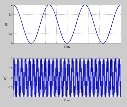
Figure 5. The function g(t) for μ = 1 (top) and the sinusoidal carrier wave (bottom).

 

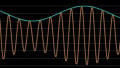
Figure 6 shows the modulated waveform along with g(t) and –g(t).

 

Figure 6. The amplitude-modulated wave (blue), the function g(t) (green), and the inverted form of g(t) (red) for μ = 1.

 

Once again, the envelope of the modulated signal is equal to g(t) = A_c(1 + μm(t)). This condition, which means that simple envelope detectors can be used for demodulation, is always true when 1 + μm(t) is positive for all values of t.

We commonly assume the maximum value of |m(t)| to be less than or equal to unity (|m(t)| ≤ 1). The condition “1 + μm(t) is positive for all t” then requires μ to be smaller than unity. To test this, let’s see what happens when we increase μ = 1.2. Figures 7 and 8 show the resulting waveforms.

 

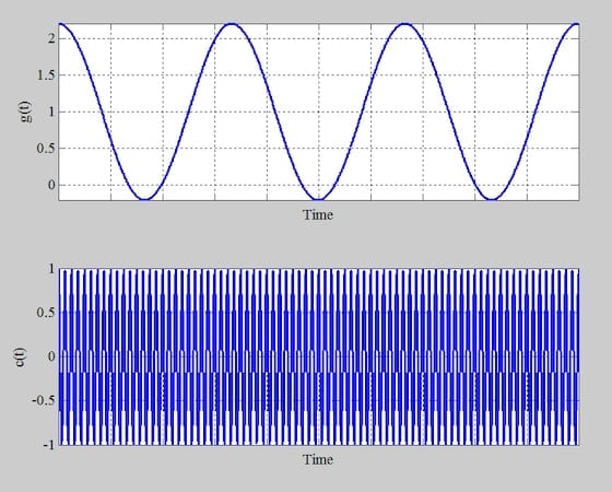
Figure 7. The function g(t) for μ = 1.2 (top) and the sinusoidal carrier wave (bottom).

 

Figure 8. The amplitude-modulated wave (blue), the function g(t) (green), and the inverted form of g(t) (red) for μ = 1.2.

 

We can see in Figure 7 that the function g(t) = 1 + μm(t) is negative for some values of t. When g(t) hits zero, a phase reversal occurs in the modulated waveform. The upper envelope therefore matches g(t) when g(t) is positive, but switches to –g(t) when g(t) is negative. In other words, the upper envelope corresponds to the absolute value of g(t). When g(t) isn’t always positive, we say that the carrier is overmodulated.

Since the envelope of the modulated waveform is no longer equal to g(t), but rather to |g(t)|, we can’t use an envelope detector for demodulation. Restoring the message signal instead requires a synchronous demodulator, which is significantly more complex. For that reason, nearly all commercial AM stations transmit conventional AM with a non-negative g(t).

Before we move on, it’s worth mentioning that the carrier frequency must be much greater than the maximum frequency of the message signal (f_c ≫ B). If this isn’t the case, an envelope—which traces the peaks of the modulated waveform—can’t be detected by the receiver.

 

Power Efficiency of Conventional AM

Given that the carrier contains no message information, we can consider its power wasted. To quantify the power efficiency of conventional amplitude modulation, we express the modulated signal (Equation 2) as:

$$s(t) ~=~ A_c \cos(\omega_c t) ~+~ A_c \mu m(t) \cos(\omega_c t)$$

Equation 3.

 

Assume that s(t) is a voltage quantity. If we place this voltage across a 1 Ω resistor, the average power delivered to the resistor is as follows:

$$P_{1 \Omega} ~=~ \lim_{T \rightarrow \infty} \frac{1}{T} \int_{-T/2}^{T/2} s^2(t) \ dt$$

Equation 4.

 

If s(t) were a periodic signal, calculating the integral over one period would be sufficient. In practice, s(t) is usually not periodic, so we need to carry out the measurement over a longer time.

Equation 5 gives us the expression for the squared message signal:

$$s^2(t) ~=~ A_c^2 \cos^2 (\omega_c t) ~+~ \big (A_c \mu m(t) \big )^2 \cos^2 (\omega_c t) ~+~ 2 A_c^2 \mu m(t) \cos^2 (\omega_c t)$$

Equation 5.

 

Consider the time average of the last term of the above equation. Applying basic trigonometric identities, we can expand the square of the cosine function as follows:

$$\begin{gather*}\lim_{T \rightarrow \infty} \frac{1}{T} \int_{-T/2}^{T/2} 2 A_c^2 \mu m(t) ~\times~ \frac{ 1 + \cos (2 \omega_c t )}{2} \ dt \\=~ A_c^2 \mu ~\times~ \lim_{T \rightarrow \infty} \frac{1}{T} \int_{-T/2}^{T/2} m(t) ~+~ m(t) \cos (2 \omega_c t ) \ dt ~=~ 0 \end{gather*}$$

Equation 6.

 

The time average of m(t) is commonly assumed to be zero, leading to the zero result we see above.

Note also that the time average of the product of two independent functions is equal to the product of their individual time averages. Since the functions m(t) and cos(2ω_ct) are independent and the time average of m(t) is zero, the time average of m(t)cos(2ω_ct) works out to zero as well. Therefore, Equation 4 simplifies to:

$$\begin{eqnarray}P_{1 \Omega} ~&=&~ \lim_{T \rightarrow \infty} \frac{1}{T} \int_{-T/2}^{T/2} A_c^2 \cos^2 (\omega_c t) ~+~ \big (A_c \mu m(t) \big )^2 \cos^2 (\omega_c t) \ dt \\&=&~ \frac{1}{2}A_c^2 ~+~ \frac{1}{2}A_c^2 \mu ^2 ~\times~ \overline{m^2(t)} \end{eqnarray}$$

Equation 7.

 

In the equation above, the bar over m²(t) denotes its time average. While the first term gives the carrier power (P_c), the second term quantifies the power of the information-bearing signal component (the sideband power, or P_s).

We intend to transmit the message information that resides in P_s. P_c is used only to make demodulation more convenient. Based on that, we can now calculate the power efficiency:

$$\eta ~=~ \frac{P_s}{P_c ~+~ P_s} ~=~ \frac{\frac{1}{2}A_c^2 \mu^2 ~\times~ \overline{m^2(t)}}{\frac{1}{2}A_c^2 ~+~ \frac{1}{2}A_c^2 \mu ^2 ~\times~ \overline{m^2(t)}}~=~\frac{\mu ^2 ~\times~ \overline{m^2(t)}}{1 ~+~ \mu ^2 ~\times~ \overline{m^2(t)}}$$

Equation 8.

 

To gain insight into the above equation, let’s assume that the message signal is a single-tone sinusoid given by m(t) = cos(ω_mt). The time average of m²(t) is therefore 0.5, producing:

$$\eta ~=~ \frac{P_s}{P_c ~+~ P_s} ~=~\frac{\mu ^2 }{2 ~+~ \mu ^2}$$

Equation 9.

 

Equation 9 shows that the efficiency increases with μ. We know that the modulation index (μ) needs to be a positive value less than or equal to unity (0 ≤ μ ≤ 1). The maximum efficiency therefore occurs at μ = 1, which is equal to η = 33%.

This means that for a single-tone sinusoidal message under the best conditions (μ = 1), only one-third of the transmitted power is used for carrying the message information. Smaller values of the modulation index further degrade the efficiency. With μ = 0.5, for example, the efficiency reduces to 11.11%. The reduction in power efficiency is the trade-off for having simpler receiver hardware.

 

Wrapping Up

As with the DSB-SC article, we’ll finish up by with a list of key takeaways from our discussion:

• In conventional AM, the transmitter sends the carrier along with the modulated signal.
• The receiver doesn’t need to generate the carrier, simplifying its hardware design and lowering the associated costs.
• The carrier power is wasted, leading to a reduction in power efficiency.
• With 100 percent modulation (μ = 1), the total power in the sidebands is one-third the total power carried by the modulated wave (η = 33%).

In the next few articles of this series, we’ll turn our attention from modulation techniques to modulator circuits, starting with the square-law modulator.

 

This article is Part 3 of a series on amplitude modulation in RF systems. A complete list of articles in this series is provided below:

1. Introduction to Modulation Techniques in RF Systems
2. Understanding Double-Sideband Suppressed-Carrier Modulation
3. Understanding Conventional Amplitude Modulation
4. Understanding the Square-Law Modulator for Generating AM Signals
5. Introduction to the Balanced Modulator for AM Signals
6. How Do Switching Modulators Generate AM Signals?
7. Understanding How Ring Modulators Produce AM Signals
8. Four Interesting AM Modulation Circuits You Should Know About
9. Demodulating Double-Sideband AM Signals
10. Introduction to Single-Sideband Modulation: The Filter Method
11. The Phasing Method and Hilbert Transforms for Single-Sideband Modulation
12. A Visual Approach to Understanding the Phasing Method for SSB Modulation
13. How Phasors Help Us Understand Bandpass Signals
14. Introduction to Weaver’s Method for SSB Signal Generation
15. Exploring the Operation of the Weaver Modulator for Single-Sideband Modulation

 

All images used courtesy of Steve Arar