A Visual Approach to Understanding the Phasing Method for SSB Modulation

Previous articles in this series introduced the filtering and phasing methods for generating single-sideband (SSB) signals. In this article, we’ll delve more deeply into the phasing method by exploring how it alters both the real and imaginary parts of the input signal’s spectrum. Unlike our earlier discussion, which examined the phasing method primarily from a mathematical viewpoint, we’ll use graphical representations to bolster our understanding.

 

Spectrum of a Real Signal

Consider a real-valued message signal to be transmitted as an SSB wave. The Fourier transform of a real-valued function exhibits conjugate symmetry, which means that the real part of the spectrum is an even function and the imaginary part is an odd function. This is illustrated in the two halves of Figure 1.

 

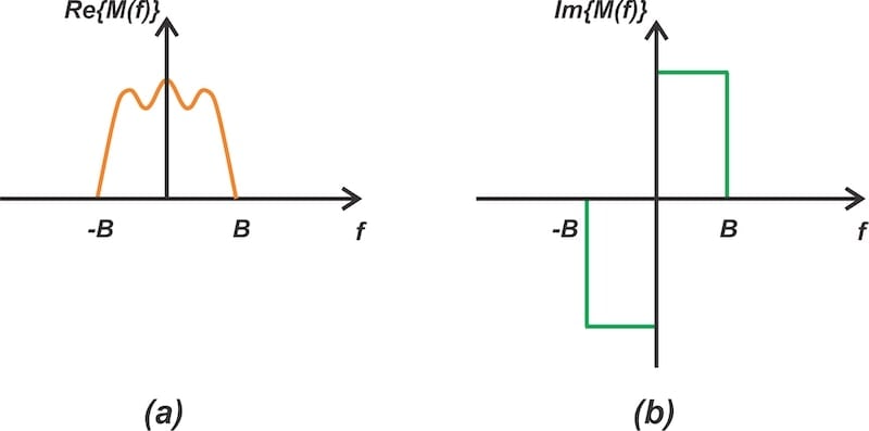
Figure 1. The real (a) and imaginary (b) parts of a real-valued baseband signal’s spectrum. Image used courtesy of Steve Arar

 

Figure 2 shows a three-dimensional representation for the above spectrum. The 3D diagram allows us to represent the spectrum at different nodes within the phasing modulator.

 

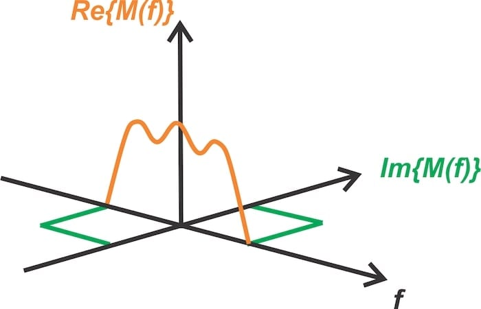
Figure 2. Demonstration of the signal spectrum using a 3D diagram. Image used courtesy of Steve Arar

 

Let’s start by using this model to visualize the Hilbert transform.

 

Illustrating the Hilbert Transform

The Hilbert transform is at the heart of the phasing method. As we learned in the previous article, it corresponds to a linear filter with the following frequency response:

$$H(f) ~=~ \begin{cases} \begin{array}{rc}j && f ~<~ 0 \\0 && f ~=~ 0 \\-j && f ~>~ 0 \end{array}\end{cases}$$

Equation 1.

 

It shifts all positive frequency components by –90 degrees, and all negative frequency components by +90 degrees. The Hilbert transform doesn’t affect the spectral amplitudes.

Since the Hilbert transform multiplies the frequency components by the imaginary unit j, it converts a real component to an imaginary one and vice versa. Figure 3 illustrates how the spectrum shown in Figure 2 is altered as it goes through the Hilbert transform.

 

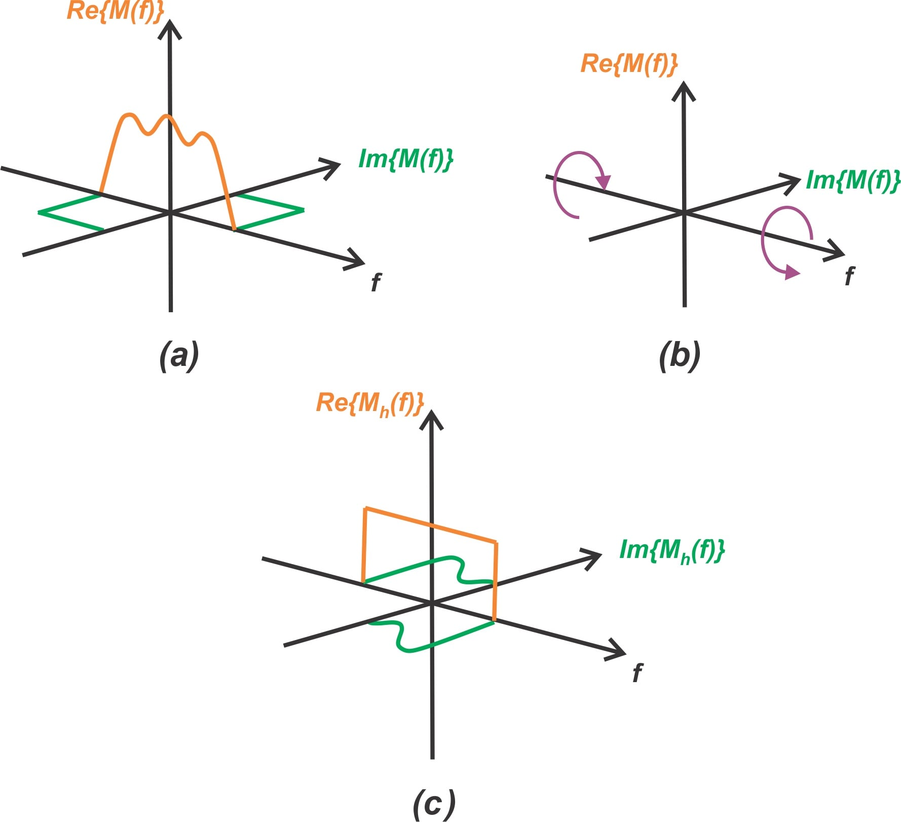
Figure 3. The input signal’s spectrum (a), the space rotation by one quadrant due to the Hilbert transform (b), and the Hilbert transform’s output spectrum (c). Image used courtesy of Steve Arar [click to enlarge]

 

We see above that the Hilbert transform rotates the positive-frequency and negative-frequency portions of the space in opposite directions by 90 degrees. To ensure that we’re not confusing the direction of the rotation for these two portions of the space, let’s examine a couple of examples.

Consider the point M(f₁) = 1 + j, where f₁ is a positive frequency. Both the real and imaginary parts of the input spectrum are positive. Because f₁ is a positive frequency component, the Hilbert transform multiplies this value by –j, producing the following:

$$M_h (f)~=~-j(1~+~j)~=~-j~-~j^2~=~1~-~j$$

Equation 2.

 

From this, we see that the output at this frequency point should have a positive real value and a negative imaginary part. This is consistent with Figure 3(b).

Next, let’s consider a negative frequency component (f₂) with positive real value and negative imaginary value: M(f₂) = 1 – j. This point corresponds to the negative-frequency portion of Figure 3(a). The Hilbert transform would produce:

$$M_h (f)~=~+j(1~-~j)~=~j~-~j^2~=~1~+~j$$

Equation 3.

 

Here, both the real and imaginary parts of the output are positive. This is once again consistent with the above diagram.

 

The Shifting Property and the Phasing Modulator

Now that we know how the Hilbert transform alters the input spectrum, let’s improve our understanding of the phasing modulator’s operation. To do so, we need to brush up on an important property of the Fourier transform. Known as the shifting property, it states that multiplying a time-domain signal by a complex exponential gives us the following:

$$e^{j \omega_0 t} x(t) \quad \overset{\text{FT}}{\longleftrightarrow} \quad X(\omega ~-~ \omega_0)$$

Equation 4.

 

where:

x(t) is the time-domain signal

X(f) is the Fourier transform of x(t)

ω₀ is a constant frequency.

In other words, the frequency spectrum is shifted by a constant frequency (ω₀).

Keeping the above in mind, let’s examine the phasing modulator block diagram in Figure 4.

 

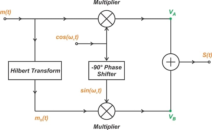
Figure 4. The functional block diagram of the SSB phasing method. Image used courtesy of Steve Arar

 

V_A and V_B denote the signals at the outputs of the upper and lower paths, respectively. We’ll also refer to these two points on the diagram as node A and node B.

First, consider the upper signal path. Using Euler's formula, the cosine local oscillator wave cos(ω_ct) can be expressed as:

$$\cos( \omega_c t) ~=~ \frac{1}{2} (e^{j \omega_c t} ~+~ e^{-j \omega_c t} )$$

Equation 5.

 

Based on the shifting property, the upper multiplier in Figure 4 translates the message spectrum by ±ω_c and scales the amplitude by a factor of 0.5. The spectrum that results can be seen (without amplitude scaling) in Figure 5(a).

Meanwhile, the sine wave input to the lower path’s local oscillator can be expressed as:

$$\sin( \omega_c t) ~=~ \frac{1}{2j} (e^{j \omega_c t} ~-~ e^{-j \omega_c t} )$$

Equation 6.

 

The lower path mixes the Hilbert transform of the message signal with the above complex exponential terms to produce V_B. To help us visualize this, let’s examine V_B’s spectrum in Figure 5(b) before we continue. You may want to open this image in a new tab.

 

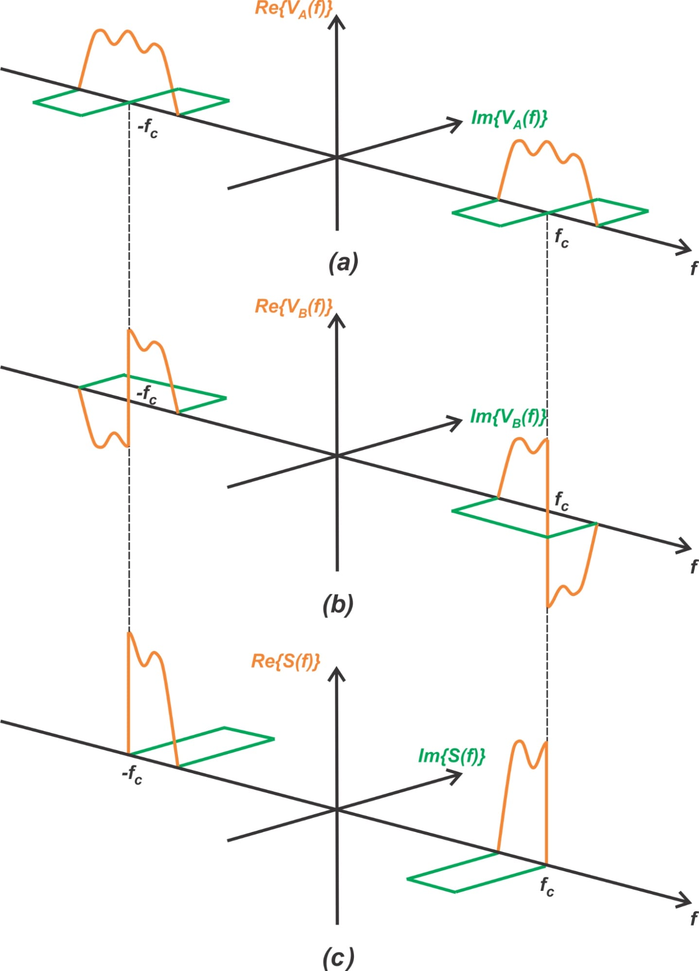
Figure 5. The spectrum produced by the upper multiplier (a), the spectrum produced by the lower multiplier (b), and the combined spectrum produced by the output summer (c). Image used courtesy of Steve Arar [click to enlarge]

 

The first term in Equation 6 shifts the output spectrum of the Hilbert transform (M_h(f) from Figure 3(c)) to be centered at ω_c, with a scaling factor of 1/2j. Division by the imaginary unit j corresponds to a phase shift of –90 degrees, producing the positive frequency portion of the output spectrum in Figure 5(b).

Dividing by j also changes the roles of the real and imaginary parts. The real parts of M_h(f) are converted to imaginary parts at node B, and the imaginary parts to real ones.

The second exponential term in Equation 6 moves the output spectrum of the Hilbert transform to –ω_c and scales it by a factor of –1/2j = j/2. Considering only the scaling factor j, we observe that the output spectrum is shifted by +90 degrees. In our 3D representation, this corresponds to a space rotation of one quadrant in a clockwise direction. Once again, note that a space rotation by one quadrant changes the real part to an imaginary part and vice versa.

 

The Modulated Output Spectrum

The modulator circuit produces the output by adding the spectrums of nodes A and B together. In this case, that means a lower-sideband signal. If we replaced the adder at the circuit’s output with a subtractor, it would generate the upper sideband instead.

The lower sidebands are of the same amplitude and polarity. Adding them together results in an output with a scale factor of two, as depicted in Figure 5(c). For the upper sidebands, both the real and imaginary parts are of the same amplitude but opposite polarity. The addition cancels them out.

 

Other Ways of Understanding the Phasing Method

In this article, we examined both the real and imaginary parts of the message signal and their modifications by the phasing modulator circuit. However, some explanations of the phasing method consider only the real part of the signal spectrum.

Consider Figure 6, for example. Taken from “The Design of CMOS Radio-Frequency Integrated Circuits,” an excellent book on RF design by Thomas H. Lee, it shows how the real part changes as it passes through the circuit.

 

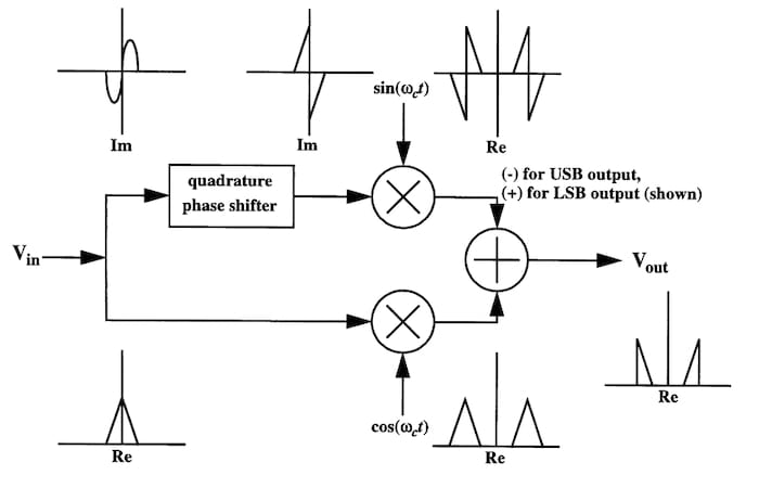
Figure 6. The phasing method of SSB signal generation when only the real part of the input spectrum is considered. Image used courtesy of Thomas H. Lee

 

Though this approach simplifies the explanation of the circuit’s operation, a thorough analysis of the phasing method should include both the real and imaginary parts of the spectrum. Now that you’ve explored the detailed explanation of this SSB circuit, attempt to verify the different spectrums illustrated in Dr. Lee’s diagram as an exercise.

 

This article is Part 12 of a series on amplitude modulation in RF systems. A complete list of articles in this series is provided below:

1. Introduction to Modulation Techniques in RF Systems
2. Understanding Double-Sideband Suppressed-Carrier Modulation
3. Understanding Conventional Amplitude Modulation
4. Understanding the Square-Law Modulator for Generating AM Signals
5. Introduction to the Balanced Modulator for AM Signals
6. How Do Switching Modulators Generate AM Signals?
7. Understanding How Ring Modulators Produce AM Signals
8. Four Interesting AM Modulation Circuits You Should Know About
9. Demodulating Double-Sideband AM Signals
10. Introduction to Single-Sideband Modulation: The Filter Method
11. The Phasing Method and Hilbert Transforms for Single-Sideband Modulation
12. A Visual Approach to Understanding the Phasing Method for SSB Modulation
13. How Phasors Help Us Understand Bandpass Signals
14. Introduction to Weaver’s Method for SSB Signal Generation
15. Exploring the Operation of the Weaver Modulator for Single-Sideband Modulation