Introduction to Weaver’s Method for SSB Signal Generation

Single-sideband (SSB) modulation is a type of amplitude modulation (AM) that uses either the lower or upper sideband to transmit information. Compared to other forms of AM, the main advantage of SSB modulation is its economy of bandwidth and power. Previous articles in this series discussed the filter method and the phasing method of SSB signal generation. Now, we’ll explore a third option: the Weaver modulator.

 

The ‘Third Method’

The filter method is the oldest and most straightforward form of SSB modulation. However, it requires bandpass filters with extremely sharp transition regions. Following its introduction in 1924, the phasing method—which eliminates this requirement—stood out as considerably superior. As illustrated in Figure 1, the phasing method generates SSB signals using a phase-shift network at the modulator’s input.

 

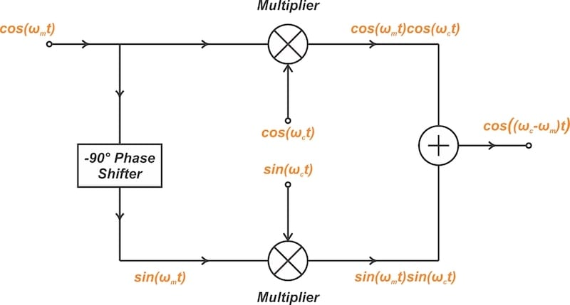
Figure 1. Generating an SSB signal with the phasing method.

 

The phase-shift networks used in this method must generate signals that are precisely 90 degrees out of phase with each other. Though simpler to implement than the aforementioned sharp bandpass filters, these are not trivial to realize. Despite that, the phasing method remained the leading approach until the late 1950s.

In 1956, Donald K. Weaver introduced a new method in a paper titled "A Third Method of Generation and Detection of Single Sideband Signals.” This method did away with the need for either sharp bandpass filters or precise phase shifters. Instead, Weaver replaced the quadrature phase shifter of the phasing method with a quadrature heterodyning process. The Weaver modulator (Figure 2) uses four multipliers and two lowpass filters.

 

Figure 2. Weaver’s method for generating SSB signals.

 

Note that Figure 2 shows the arrangement for keeping the upper sideband (USB). Later on in the article, we'll explore the modifications needed to produce the lower sideband (LSB) instead.

In Weaver’s circuit, the required 90-degree phase difference is generated by the first set of multipliers together with the lowpass filters. The second set of multipliers in Weaver’s circuit operates in the same manner as in the phasing method, except that they use different local oscillator frequencies.

The first pair of multipliers in this circuit downconverts the message signal with an oscillator whose frequency (f₀) is in the center of the message signal’s frequency range. If the message signal is limited to the frequency band f_a ≤ f ≤ f_b, the carrier applied to the first pair of multipliers is:

$$f_{0} ~=~ \frac{f_a ~+~ f_b}{2}$$

Equation 1.

 

After downconversion, the message signal’s center frequency is now DC (f = 0). The resulting signals are then passed through lowpass filters with a cutoff frequency of:

$$f_{cutoff} ~=~ \frac{f_b ~-~ f_a}{2}$$

Equation 2.

 

The carrier applied to the second pair of multipliers has a frequency greater than f_cutoff. If the desired carrier frequency is f_c, then the second pair of multipliers must be driven by oscillators with frequency f_c + f₀.

 

Applying a Single-Tone Input to the Weaver Modulator

Let’s use Figure 3 to analyze the circuit’s response to a single-frequency message, m(t) = cos(ω_mt).

 

Figure 3. Applying a single-frequency input to the Weaver modulator.

 

Using a basic trigonometric identity, we obtain the output of the upper multiplier:

$$\cos( \omega_m t) \cos( \omega_0 t) ~=~ \frac{1}{2} \big [ \cos \big ( ( \omega_m ~+~ \omega_0)t \big ) ~+~ \cos \big ( ( \omega_m ~-~ \omega_0)t \big ) \big ]$$

Equation 3.

 

The first term inside the square brackets is at a higher frequency and can be eliminated by a lowpass filter. At the output of the upper lowpass filter (node A), we therefore have:

$$v_A ~=~ Lowpass \big [ \cos( \omega_m t) \cos( \omega_0 t) \big ] ~=~ \frac{1}{2} \cos \big ( ( \omega_m ~-~ \omega_0)t \big )$$

Equation 4.

 

The lower path in the circuit diagram multiplies the input by a sine wave. The output of this multiplier is:

$$\cos( \omega_m t) \sin( \omega_0 t) ~=~ \frac{1}{2} \big [ \sin \big ( ( \omega_m ~+~ \omega_0)t \big ) ~-~ \sin \big ( ( \omega_m ~-~ \omega_0)t \big ) \big ]$$

Equation 5.

 

The high-frequency component is eliminated as the signal passes through the lowpass filter, producing the following signal at node B:

$$v_B ~=~ Lowpass \big [ \cos( \omega_m t) \sin( \omega_0 t) \big ] ~=~ -\frac{1}{2} \sin \big ( ( \omega_m ~-~ \omega_0)t \big )$$

Equation 6.

 

Equations 4 and 6 indicate that the output signals from the lowpass filters exhibit a phase difference of 90 degrees. As you may recall, creating this phase difference was the key challenge of the phasing method.

We’re now ready to find the output signal of the modulator. Using v_A and v_B, the output signal from the Weaver modulator is:

$$s_{out} ~=~ \underset{v_A}{\underbrace{\frac{1}{2} \cos \big ( ( \omega_m ~-~ \omega_0)t \big )}} ~\times~ \cos \big ( ( \omega_c ~+~ \omega_0)t \big ) \underset{v_B}{\underbrace{~-~\frac{1}{2} \sin \big ( ( \omega_m ~-~ \omega_0)t \big )}} ~\times~ \sin \big ( ( \omega_c ~+~ \omega_0)t \big )$$

Equation 7.

 

We can simplify this expression by recognizing its similarities to the following trigonometric identity:

$$\cos (A~+~B) ~=~ \cos(A) \cos(B) ~-~ \sin(A) \sin(B)$$

Equation 8.

 

Applying this identity, the output signal simplifies to:

$$\begin{eqnarray}s_{out} &~=~& \frac{1}{2} \cos \big ( ( \omega_m ~-~ \omega_0)t ~+~ ( \omega_c ~+~ \omega_0)t \big ) \\&~=~& \frac{1}{2} \cos \big ( ( \omega_m ~+~ \omega_c)t \big )\end{eqnarray}$$

Equation 9.

 

The spectrum of this signal consists of two impulses at ±(f_c + f_m). These correspond to the upper-sideband components in Figure 4.

 

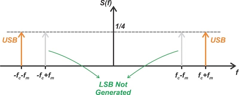
Figure 4. The output spectrum of the Weaver modulator for a single-frequency message signal.

 

Generating LSB Signals

So far, we’ve only used the Weaver modulator to generate USB signals. By altering the polarity of specific terms, however, we can eliminate the upper sideband and create LSB signals instead. Figure 5 demonstrates the required adjustments.

 

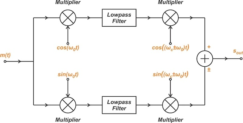
Figure 5. Weaver’s circuit can generate either upper or lower SSB signals.

 

As we know from our earlier discussion, adding the upper and lower path signals together produces the upper sideband signal. To produce the lower sideband signal, we instead subtract the lower path signal from the upper path. This changes Equation 7 to:

$$s_{out} ~=~ \underset{v_A}{\underbrace{\frac{1}{2} \cos \big ( ( \omega_m ~-~ \omega_0)t \big )}} ~\times~ \cos \big ( ( \omega_c ~-~ \omega_0)t \big )~-~ \big [ \underset{v_B}{\underbrace{-\frac{1}{2} \sin \big ( ( \omega_m ~-~ \omega_0)t \big )}} \big ] ~\times~ \sin \big ( ( \omega_c ~-~ \omega_0)t \big )$$

Equation 10.

 

which simplifies to:

$$\begin{eqnarray}s_{out} &~=~& \frac{1}{2} \cos \big ( ( \omega_m ~-~ \omega_0)t ~-~ ( \omega_c ~-~ \omega_0)t \big ) \\&~=~& \frac{1}{2} \cos \big ( ( \omega_m ~-~ \omega_c)t \big )\end{eqnarray}$$

Equation 11.

 

The spectrum of this signal consists of two impulses at –f_c + f_m and f_c – f_m, corresponding to the LSB components (see Figure 4).

 

Using the Complex Baseband Representation to Understand Weaver’s Method

In the previous article, we learned about the complex baseband representation of bandpass signals. Let's briefly revisit some key aspects of this concept that are relevant to our current discussion. This will allow us to deepen our comprehension of the Weaver modulator by examining it from another angle.

Consider a modulated sinusoidal wave centered at a fixed RF frequency (f_c) with a slowly varying amplitude and phase:

$$s_{RF}(t) ~=~ A(t) \cos \big ( \omega_c t ~+~ \theta(t) \big )$$

Equation 12.

 

where A(t) and θ(t) are the instantaneous amplitude and phase, respectively, of the time-varying signal. The above equation can be rewritten as:

$$s_{RF}(t) ~=~ Re \Big \{ \big [A(t) e^{j \theta(t)} \big ] e^{j \omega_c t} \Big \}$$

Equation 13.

 

The term inside the square brackets is the complex baseband representation of the signal:

$$s_l (t) ~=~ A(t) e^{j \theta(t)}$$

Equation 14.

 

The above equation can also be expressed in Cartesian form:

$$s_l(t) ~=~ s_i(t) ~+~ j s_q (t)$$

Equation 15.

 

where s_i(t) and s_q(t) are the real-valued in-phase and quadrature components of s_l(t). From Equations 14 and 15, we obtain the following values for the in-phase and quadrature components:

$$s_i(t) ~=~ A(t) \cos ( \theta) \quad \text{and} \quad s_q(t)~=~A(t) \sin( \theta)$$

Equation 16.

 

This analysis illustrates that a bandpass signal can be decomposed into two lowpass signals that are 90 degrees out of phase. The pertinent question is this: how can we generate s_i(t) and s_q(t) for a given signal? To find out, let’s turn our attention back to the circuits.

 

Building Blocks of the Weaver Modulator

As we discussed in the previous article, the in-phase and quadrature components of the baseband representation can be obtained by a pair of multipliers and lowpass filters. This circuit is illustrated in Figure 6.

 

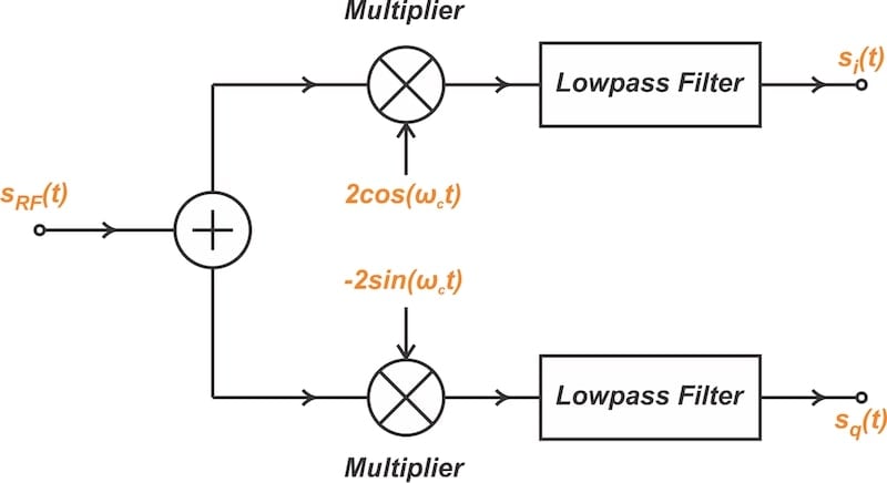
Figure 6. The circuit that generates lowpass in-phase and quadrature signals from the bandpass signal.

 

Furthermore, if we have the in-phase and quadrature components, we can reconstruct the bandpass signal using the arrangement in Figure 7.

 

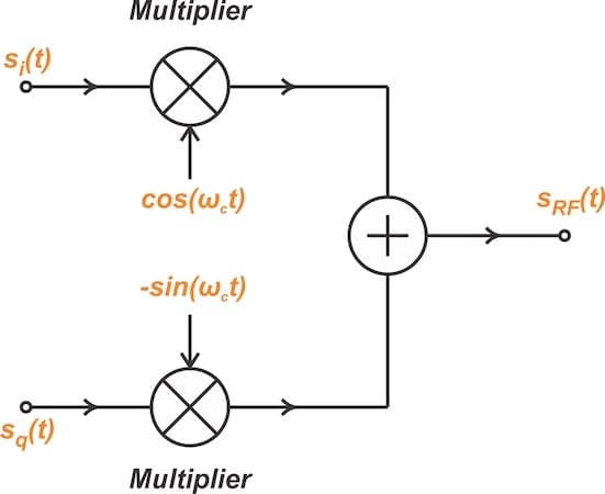
Figure 7. The circuit that generates the bandpass signal from the lowpass in-phase and quadrature signals.

 

The circuits in Figures 6 and 7 are the building blocks of the Weaver modulator. In the combined circuit, the two pairs of multipliers are driven by different local oscillator frequencies. For instance, the first pair of multipliers are driven by f₀, whereas the second pair is driven by f_c + f₀ for upper sideband generation. If both multiplier pairs used the same oscillator frequency, the circuit would actually reproduce the message signal at the output.

Typically, when discussing the concept of complex baseband representation, the input is an RF signal. However, Weaver’s circuit applies this concept to a baseband signal. The Weaver modulator does this by downconverting the message signal to find its in-phase and quadrature components.

 

Wrapping Up

The Weaver modulator requires neither the sharp bandpass filters of the filter method nor the precise phase-shifters of the phasing method. It’s also versatile enough to perform functions beyond generating SSB signals. For instance, it can be adapted to function as an SSB demodulator by altering the sequence of frequency conversions within the circuit.

The circuit's proper operation depends on the following conditions being met:

• The oscillator signals must be exactly in quadrature.
• The oscillator signals must have equal amplitudes.
• The gains of the upper and lower paths must match.

In the next article, we’ll study how an arbitrary input spectrum changes as it passes through the Weaver modulator.

 

This article is Part 14 of a series on amplitude modulation in RF systems. A complete list of articles in this series is provided below:

1. Introduction to Modulation Techniques in RF Systems
2. Understanding Double-Sideband Suppressed-Carrier Modulation
3. Understanding Conventional Amplitude Modulation
4. Understanding the Square-Law Modulator for Generating AM Signals
5. Introduction to the Balanced Modulator for AM Signals
6. How Do Switching Modulators Generate AM Signals?
7. Understanding How Ring Modulators Produce AM Signals
8. Four Interesting AM Modulation Circuits You Should Know About
9. Demodulating Double-Sideband AM Signals
10. Introduction to Single-Sideband Modulation: The Filter Method
11. The Phasing Method and Hilbert Transforms for Single-Sideband Modulation
12. A Visual Approach to Understanding the Phasing Method for SSB Modulation
13. How Phasors Help Us Understand Bandpass Signals
14. Introduction to Weaver’s Method for SSB Signal Generation
15. Exploring the Operation of the Weaver Modulator for Single-Sideband Modulation

 

All images used courtesy of Steve Arar