Introduction to Single-Sideband Modulation: The Filter Method

So far in this series, we’ve explored two methods of amplitude modulation (AM):

• Double-sideband suppressed carrier (DSB-SC).
• Conventional AM.

These techniques transmit both the upper and lower sidebands of a message signal. For example, Figure 1 shows a typical DSB-SC output spectrum.

 

Figure 1. The spectrum of the baseband message signal (a) and that of the DSB-SC signal (b). The upper and lower sidebands are denoted by USB and LSB, respectively. Image used courtesy of Steve Arar

 

Because the modulated signal includes both sidebands, it occupies twice the bandwidth of the message signal.

To use bandwidth more efficiently, single-sideband (SSB) modulation eliminates either the upper or lower sideband. Like DSB-SC, this type of AM also suppresses the carrier wave. For that reason, it’s sometimes referred to as SSB-SC modulation.

The primary advantage of SSB modulation is that it requires only half the bandwidth of double-sideband (DSB) modulation. Because SSB signals occupy a narrower bandwidth, the amount of noise in the signal is also reduced. With an SSB receiver, the intercepted noise bandwidth is equal to the bandwidth of the message signal. A DSB receiver, on the other hand, captures the noise from twice the signal bandwidth.

This difference in intercepted noise bandwidth affects the achievable signal-to-noise ratio (SNR), making SSB more energy-efficient for the same signal power. The effective SNR of a DSB signal is half the effective SNR of SSB when the signal power is the same.

Over the next few articles, we’ll discuss three established methods of generating SSB signals:

1. The filter method.
2. The phasing method.
3. Weaver’s method (sometimes just referred to as the third method).

This article will cover the filter method, which involves generating a DSB-SC signal and then filtering out the unwanted sideband. The filter method is particularly appealing for message signals with minimal low-frequency content. Since frequencies below about 300 Hz aren’t essential for voice signal intelligibility, it’s often utilized in speech transmission.

 

The Basic Filter Method

Figure 2 shows the most straightforward method for generating SSB signals. Note that the multiplier can be implemented using a balanced modulator.

 

Figure 2. Generating SSB signals by using a bandpass filter to retain only the desired sideband. Image used courtesy of Steve Arar

 

The multiplier produces a DSB-SC signal that subsequently passes through a highly selective bandpass filter. The filter selects one sideband—either upper or lower—while rejecting the other. Figure 3(b) shows the ideal filter response for passing the upper sideband (USB) of the DSB signal in Figure 3(a).

 

Figure 3. The spectrum of the DSB signal (a) and the ideal filter response for generating an upper-sideband SSB signal (b). Image used courtesy of Steve Arar

 

As illustrated above, the filter should ideally cut off abruptly at the carrier frequency (f_c). However, real-world filters can’t achieve perfect brick-wall selectivity—a gentle transition band is unavoidable. A practical filter may therefore suppress some of the desired sideband or allow some of the undesired sideband to pass through to the output.

Luckily, many practical signals—including speech—exhibit minimal energy near zero frequency. The result is a gap in the DSB signal spectrum around the carrier frequency, where the bandpass filter's transition band is located. This is illustrated in Figure 4.

 

Figure 4. Spectrum of a message signal with an energy gap around zero frequency (a) and the DSB-SC signal at the output of the multiplier (b). Image used courtesy of Steve Arar

 

In the above figure, f_a is the lowest frequency component of the message signal. This leads to an energy gap centered at f_c in the DSB signal. The purple curve in Figure 4(b) shows the required filter response for retaining the upper sideband.

The desired sideband must lie inside the passband of the filter; the unwanted sideband must lie inside the filter’s stopband. The filter's transition band therefore spans from f_c + f_a to f_c – f_a. In other words, the transition band of the filter is 2f_a, or twice the lowest frequency component contained in the message signal.

Although the energy gap in the input spectrum around zero frequency relaxes the sideband filter requirements somewhat, we may still need sharp filters to eliminate the unwanted sideband. Furthermore, the achievable transition region of a practical filter depends on the cutoff frequency as well as the filter order. High-frequency, sharp filters generally require higher-Q components and are more susceptible to component non-idealities.

To get around the need for these filters, we add an extra step to the filtering process. We’ll discuss this in the next section, using the transmission of analog voice signals—one of SSB modulation’s primary applications—as an example.

 

The Two-Step Filter Method

In voice transmission, the lowest frequency component present in the signal is about 30 Hz. However, to ease the filter requirements, we commonly assume that the lowest frequency of the speech signal is 300 Hz. The bandpass filter should therefore have a transition band of 600 Hz.

As a rule of thumb, the achievable transition region for a practical filter is about 1% of its cutoff frequency. Based on that, the cutoff frequency is about 60 kHz. In other words, if the available transition band of the filter is 600 Hz, sideband filter considerations limit the maximum carrier frequency to about 60 kHz.

When the carrier frequency is significantly above 60 kHz, filter design becomes more complex. Figure 5 illustrates the two-step frequency translation process we use in such cases.

 

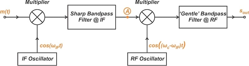
Figure 5. SSB signal generation using a two-stage process with an intermediate frequency. Image used courtesy of Steve Arar

 

First, we generate a DSB-SC signal at a low intermediate frequency (f_IF) that’s much smaller than the target carrier (f_c). A sharp sideband filter, which is easier to implement at low frequencies, is applied to the DSB signal to create an SSB-SC signal at f_IF.

To obtain the signal spectrum at the output of the IF filter (node A in Figure 5), we can use the results of Figure 4(b). Assuming that the IF filter retains the upper sidebands while suppressing the lower ones, the resultant SSB signal at node A is shown in Figure 6.

 

Figure 6. Signal spectrum at the output of the IF filter. Image used courtesy of Steve Arar

 

The signal at node A can be viewed as a message signal with an energy gap of 2f_IF + 2f_a ≈ 2f_IF around zero frequency. This signal is then applied to the second stage for modulation to the desired carrier frequency. Since the energy gap for the signal applied to the second multiplier has increased to 2f_IF, a bandpass filter with a much gentler roll-off can be used in the second stage.

Due to their low cost and simplicity of design, crystal filters are the predominant choice for SSB transmitters. They also offer exceptional selectivity thanks to their high Q. However, some designs use ceramic or DSP filters instead.

 

When Not to Use SSB Modulation

SSB modulation isn’t recommended for digital data or pulse transmission. To understand why, we need to learn a little bit about the time representation of SSB signals. SSB signals can be described in the time domain as follows:

$$s(t) ~=~ m(t) \cos(\omega_c t) ~\pm~ m_h(t) \sin(\omega_c t)$$

Equation 1.

 

where m_h(t) is the Hilbert transform of m(t), the message signal. The plus sign produces the lower sidebands; the minus sign produces the upper sidebands. The above equation shows that the envelope of the SSB signal is given by:

$$R(t) ~=~ \sqrt{ m^2(t) ~+~ m^2_h(t)}$$

Equation 2.

 

A well-known property of the Hilbert transform is that it exhibits sharp peaks at points where the message signal changes abruptly. A classic demonstration of this property involves plugging in a square wave into the Hilbert transform. The result is shown in Figure 7.

 

Figure 7. A rectangular pulse (dashed) and its Hilbert transform (solid). Image used courtesy of F. R. Kschischang

 

When the input signal has stepwise discontinuities, it produces large values at the Hilbert transform output. Practical circuits can’t easily produce the large peaks for the Hilbert transform, making SSB modulation unsuitable for pulse and digital data signals. To smooth out unwanted high-frequency input transitions and avoid generating large peaks, even speech signals may need to be low-pass filtered before being applied to an SSB transmitter.

 

Wrapping Up

SSB modulation improves on DSB modulation by eliminating one of the redundant sidebands, reducing the transmission bandwidth by a factor of two. However, the filter method of generating SSB signals requires sideband filters with extremely sharp roll-off characteristics. This is difficult to achieve, especially at high frequencies.

Sharp filters are generally more effective and easier to design at lower frequencies. To take advantage of this, we first generate a DSB signal at an intermediate frequency and then filter it. This two-step frequency translation process allows for more precise selection of the desired sideband.

The filter method isn’t the only way of generating SSB signals, however—just the oldest and most straightforward. In the next article, we’ll discuss the phasing method, which removes the requirement for a sharp filter. We’ll also learn more about the Hilbert transform.

 

This article is Part 10 of a series on amplitude modulation in RF systems. A complete list of articles in this series is provided below:

1. Introduction to Modulation Techniques in RF Systems
2. Understanding Double-Sideband Suppressed-Carrier Modulation
3. Understanding Conventional Amplitude Modulation
4. Understanding the Square-Law Modulator for Generating AM Signals
5. Introduction to the Balanced Modulator for AM Signals
6. How Do Switching Modulators Generate AM Signals?
7. Understanding How Ring Modulators Produce AM Signals
8. Four Interesting AM Modulation Circuits You Should Know About
9. Demodulating Double-Sideband AM Signals
10. Introduction to Single-Sideband Modulation: The Filter Method
11. The Phasing Method and Hilbert Transforms for Single-Sideband Modulation
12. A Visual Approach to Understanding the Phasing Method for SSB Modulation
13. How Phasors Help Us Understand Bandpass Signals
14. Introduction to Weaver’s Method for SSB Signal Generation
15. Exploring the Operation of the Weaver Modulator for Single-Sideband Modulation

 

Featured image used courtesy of Adobe Stock; background of featured image used courtesy of Steve Arar